
In the part – 1, we’ve discussed the details on the basic concept of this enw LLM frame work & how it enables the similar capability without the need for accelerated GPUs or specific hardwares. In this post, we’ll further discuss this & explore more details on top of that.
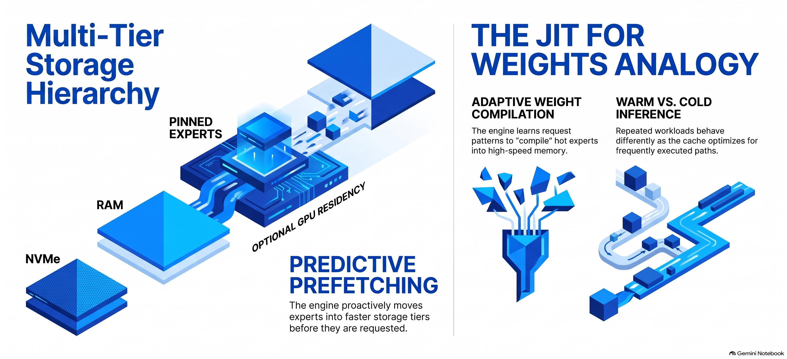
The engine records routing activity and can keep frequently used experts in faster memory. It combines mechanisms such as:
NVMe → RAM caching → pinned hot experts → optional GPU residency → prefetching
The project describes this as analogous to a JIT compiler for weights: instead of compiling frequently executed code, it learns which model experts are frequently requested and moves those experts into faster storage tiers.
This is why repeated workloads can behave differently from completely cold inference.
Colibrì can also distribute expert reads across two storage devices.
Because disk bandwidth is frequently the limiting factor, the engine supports a second model mirror and routes reads across the drives according to measured or configured bandwidth.
And, we’ll be also exploring this appraoch to reduce the load in our MacBook Pro.
So something conceptually like:
                     ┌── NVMe SSD #1
Model expert request ┤
                     └── NVMe SSD #2
                           ↓
                          RAM
                           ↓
                          GPU
This can increase the effective streaming bandwidth.
That is a fairly distinctive capability compared with conventional local LLM runtimes.
A major architecture strategy:
The API also supports persistent KV contexts.
Colibrì can save KV state to .coli_kv files and reuse the common prefix when a conversation continues. For more information please refer the following link.
That can matter enormously for huge models because repeatedly processing a long conversation history could otherwise be extremely expensive.
Multiple isolated KV slots are also supported, currently up to 16 according to the API documentation. Refer the below link to know more on this.
Limitation:
Colibrì demonstrates that enormous models can run on modest hardware.
That does not mean they run at cloud-API speeds. The project’s own benchmark documentation is unusually transparent about this.
For the 744B GLM model, documented examples include roughly:
- 25 GB development machine, cold: 0.05–0.1 tokens/s
- 128 GB CPU-only system, warm: ~1.8 tokens/s
- RTX 5070 Ti system: ~1.07 tokens/s in one documented configuration
- Large six-RTX-5090 configuration: several tokens per second with experts resident rather than coming from disk.
In Colibri, the coding agent might send 10,000–20,000 tokens before the user’s first message, and disk-streamed prefill could therefore take an extremely long time.

Colibrì’s innovation is primarily accessibility and heterogeneous resource utilization, not magically eliminating the physics of memory bandwidth.
Why this initiative is interesting?
The key contribution is not simply “running an LLM locally.” Tools such as Ollama already make that common.
Colibrì is exploring a different question:
What if model size no longer had to be constrained by available RAM or VRAM?
The repository treats storage, memory, caching, routing patterns, speculative decoding, quantization, NUMA, CPU/GPU overlap, and expert placement as parts of the inference system itself.
That could make it valuable for four broad areas:
- Local/private inference, particularly when sending data to an external inference provider is undesirable.
- AI systems research, especially research into MoE routing, caching, memory hierarchy, quantization, and heterogeneous computing.
- Low-cost experimentation with frontier-scale open models, where owning several data-center GPUs would otherwise be required.
- Building local AI services, because its OpenAI/Anthropic-compatible APIs can sit underneath applications, RAG systems, coding tools, or agent frameworks.
One qualification is important: local execution can improve control over where prompts and model execution occur, but “local” by itself should not be interpreted as an automatic security or privacy guarantee. Network exposure, APIs, applications connected to the server, file access, and logging still need to be configured appropriately. Colibrì defaults the server to localhost and recommends setting an API key before exposing it beyond the machine.
Now, let us understand how we want to proceed with our architecture implementation locally even further reducing the need for the SSD memories of my Macbook Pro.

Colibrì supports a useful feature called a partial model mirror. You can retain the complete model on your external drive like mine (SD_BLACK) and copy a selected portion of frequently used model shards onto your Mac’s much faster internal SSD. Colibrì then reads from both locations. Its official documentation provides commands to plan, stage and verify these partial mirrors. I tried both the options, partially, stored in Macbook & partially stored in my high speed SSD USB. And, alo test by placing the complete model in my MacBook Pro to understand the implications of the performance for storing them in different places.
Now, what my external drive will tell us about the performance –

I’ve used a faster SSD USB from SanDisk to get the better response, while storing the Colibri library over there. That way I can get the almost similar response from the external SSD USB like my internal Macbook Pro’s SSD.
SanDisk officially specifies the Extreme Portable SSD at up to 1,050 MB/s sequential read and 1,000 MB/s sequential write, using USB 3.2 Gen 2. For more on this device, you can refer the following link.
Let us understand, how the cache works for us –
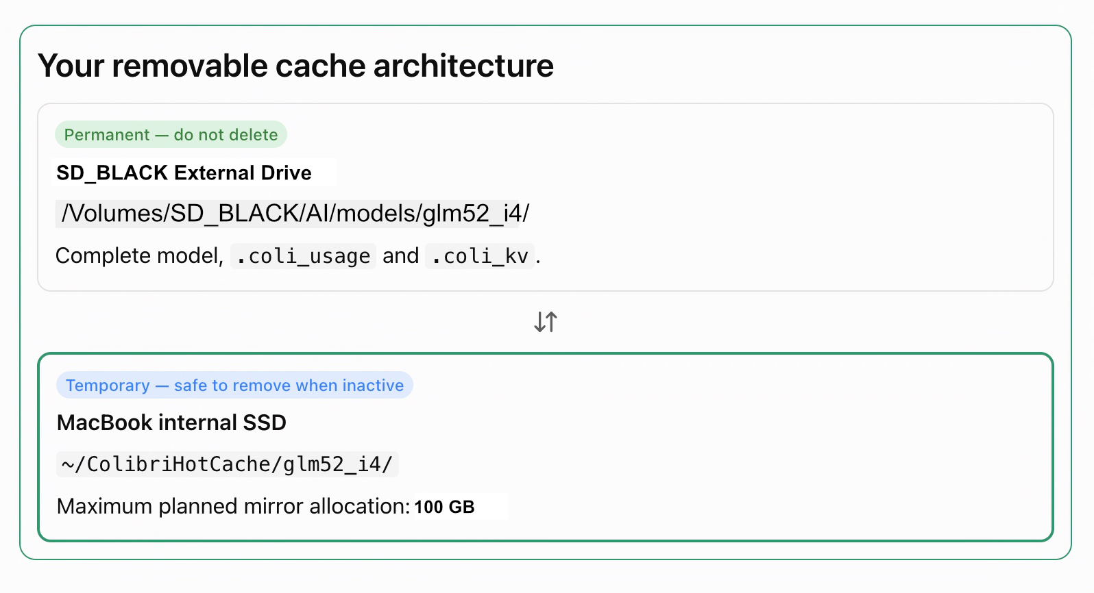
From thje above image, you can see that by default, the main models stays in the faster SanDisk SSD USB. However, 100 GB of the mirror models are kept inside the main laptop’s SSD for even better performance. So, it is a mid-level tradeoff againsts the lapotp’s memory utilization Vs performance.
Using the following way, you can configure the model endpoint ->
export COLI_MODEL="/Volumes/SD_BLACK/AI/models/glm52_i4"
export MIRROR="$HOME/ColibriMirror/glm52_i4"

df -h "$HOME"
mkdir -p "$MIRROR"

cd /Volumes/SD_BLACK/AI/colibri/c

./coli mirror plan \
  --model "$COLI_MODEL" \
  --mirror "$MIRROR" \
  --budget-gib 100 \
--reserve-gib 60Review the plan first. Provided you have sufficient internal SSD space, stage and verify the selected shards:
./coli mirror stage \
  --model "$COLI_MODEL" \
  --mirror "$MIRROR" \
  --budget-gib 100 \
  --reserve-gib 60

./coli mirror verify \
  --model "$COLI_MODEL" \
--mirror "$MIRROR"These commands are supported by the current repository; an older local Colibrì executable may need updating if it does not recognize coli mirror. Staging preserves the original external model and verifies copied shards. For more information on this, please refer to the following link.
After successful verification, start the server with the mirror enabled:
COLI_MODEL_MIRROR="$MIRROR" \
COLI_METAL=1 \
CAP_RAISE=0 \
MTP=0 \
./coli serve \
  --model "$COLI_MODEL" \
  --ram 88 \
  --cap 8 \
  --host 127.0.0.1 \
  --port 8000 \
--model-id glm-5.2-colibriNow, in the next thread we’ll understand the entire step-by-step setup of this initiative & explian one more complex combinations to get even better resolution with custom twists.
Till then, Happy Avenging! 😀
Note: All the data & scenarios posted here are representative of data & scenarios available on the internet for educational purposes only. There is always room for improvement in this kind of model & the solution associated with it. This article is for educational purposes only. The techniques described should only be used for authorized security testing and research. Unauthorized access to computer systems is illegal and unethical & not encouraged.


You must be logged in to post a comment.