Hi Guys,
Today, I’ll be demonstrating some scenarios based on open-source data from Canada. In this post, I will only explain some of the significant parts of the code. Not the entire range of scripts here.
Let’s explore a couple of sample source data –
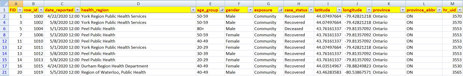
I would like to explore how much this disease caused an impact on the elderly in Canada.
Let’s explore the source directory structure –

For this, you need to install the following packages –
pip install pandas
pip install seaborn
Please find the PyPi link given below –
In this case, we’ve downloaded the data from Canada’s site. However, they have created API. So, you can consume the data through that way as well. Since the volume is a little large. I decided to download that in CSV & then use that for my analysis.
Before I start, let me explain a couple of critical assumptions that I had to make due to data impurities or availabilities.
- If there is no data available for a specific case, my application will consider that patient as COVID-Active.
- We will consider the patient is affected through Community-spreading until we have data to find it otherwise.
- If there is no data available for gender, we’re marking these records as “Other.” So, that way, we’re making it into that category, where the patient doesn’t want to disclose their sexual orientation.
- If we don’t have any data, then by default, the application is considering the patient is alive.
- Lastly, my application considers the middle point of the age range data for all the categories, i.e., the patient’s age between 20 & 30 will be considered as 25.
1. clsCovidAnalysisByCountryAdv (This is the main script, which will invoke the Machine-Learning API & return 0 if successful.)
##############################################
#### Written By: SATYAKI DE               ####
#### Written On: 01-Jun-2020              ####
#### Modified On 01-Jun-2020              ####
####                                      ####
#### Objective: Main scripts for Logistic ####
#### Regression.                          ####
##############################################

import pandas as p
import clsL as log
import datetime

import matplotlib.pyplot as plt
import seaborn as sns
from clsConfig import clsConfig as cf

# %matplotlib inline -- for Jupyter Notebook
class clsCovidAnalysisByCountryAdv:
    def __init__(self):
        self.fileName_1 = cf.config['FILE_NAME_1']
        self.fileName_2 = cf.config['FILE_NAME_2']
        self.Ind = cf.config['DEBUG_IND']
        self.subdir = str(cf.config['LOG_DIR_NAME'])

    def setDefaultActiveCases(self, row):
        try:
            str_status = str(row['case_status'])

            if str_status == 'Not Reported':
                return 'Active'
            else:
                return str_status
        except:
            return 'Active'

    def setDefaultExposure(self, row):
        try:
            str_exposure = str(row['exposure'])

            if str_exposure == 'Not Reported':
                return 'Community'
            else:
                return str_exposure
        except:
            return 'Community'

    def setGender(self, row):
        try:
            str_gender = str(row['gender'])

            if str_gender == 'Not Reported':
                return 'Other'
            else:
                return str_gender
        except:
            return 'Other'

    def setSurviveStatus(self, row):
        try:
            # 0 - Deceased
            # 1 - Alive
            str_active = str(row['ActiveCases'])

            if str_active == 'Deceased':
                return 0
            else:
                return 1
        except:
            return 1

    def getAgeFromGroup(self, row):
        try:
            # We'll take the middle of the Age group
            # If a age range falls with 20, we'll
            # consider this as 10.
            # Similarly, a age group between 20 & 30,
            # should reflect by 25.
            # Anything above 80 will be considered as
            # 85

            str_age_group = str(row['AgeGroup'])

            if str_age_group == '<20':
                return 10
            elif str_age_group == '20-29':
                return 25
            elif str_age_group == '30-39':
                return 35
            elif str_age_group == '40-49':
                return 45
            elif str_age_group == '50-59':
                return 55
            elif str_age_group == '60-69':
                return 65
            elif str_age_group == '70-79':
                return 75
            else:
                return 85
        except:
            return 100

    def predictResult(self):
        try:

            # Initiating Logging Instances
            clog = log.clsL()

            # Important variables
            var = datetime.datetime.now().strftime(".%H.%M.%S")
            print('Target File Extension will contain the following:: ', var)
            Ind = self.Ind
            subdir = self.subdir

            #######################################
            #                                     #
            # Using Logistic Regression to        #
            # Idenitfy the following scenarios -  #
            #                                     #
            # Age wise Infection Vs Deaths        #
            #                                     #
            #######################################
            inputFileName_2 = self.fileName_2

            # Reading from Input File
            df_2 = p.read_csv(inputFileName_2)

            # Fetching only relevant columns
            df_2_Mod = df_2[['date_reported','age_group','gender','exposure','case_status']]
            df_2_Mod['State'] = df_2['province_abbr']

            print()
            print('Projecting 2nd file sample rows: ')
            print(df_2_Mod.head())

            print()
            x_row_1 = df_2_Mod.shape[0]
            x_col_1 = df_2_Mod.shape[1]

            print('Total Number of Rows: ', x_row_1)
            print('Total Number of columns: ', x_col_1)

            #########################################################################################
            # Few Assumptions                                                                       #
            #########################################################################################
            # By default, if there is no data on exposure - We'll treat that as community spreading #
            # By default, if there is no data on case_status - We'll consider this as active        #
            # By default, if there is no data on gender - We'll put that under a separate Gender    #
            # category marked as the "Other". This includes someone who doesn't want to identify    #
            # his/her gender or wants to be part of LGBT community in a generic term.               #
            #                                                                                       #
            # We'll transform our data accordingly based on the above logic.                        #
            #########################################################################################
            df_2_Mod['ActiveCases'] = df_2_Mod.apply(lambda row: self.setDefaultActiveCases(row), axis=1)
            df_2_Mod['ExposureStatus'] = df_2_Mod.apply(lambda row: self.setDefaultExposure(row), axis=1)
            df_2_Mod['Gender'] = df_2_Mod.apply(lambda row: self.setGender(row), axis=1)

            # Filtering all other records where we don't get any relevant information
            # Fetching Data for
            df_3 = df_2_Mod[(df_2_Mod['age_group'] != 'Not Reported')]

            # Dropping unwanted columns
            df_3.drop(columns=['exposure'], inplace=True)
            df_3.drop(columns=['case_status'], inplace=True)
            df_3.drop(columns=['date_reported'], inplace=True)
            df_3.drop(columns=['gender'], inplace=True)

            # Renaming one existing column
            df_3.rename(columns={"age_group": "AgeGroup"}, inplace=True)

            # Creating important feature
            # 0 - Deceased
            # 1 - Alive
            df_3['Survived'] = df_3.apply(lambda row: self.setSurviveStatus(row), axis=1)

            clog.logr('2.df_3' + var + '.csv', Ind, df_3, subdir)

            print()
            print('Projecting Filter sample rows: ')
            print(df_3.head())

            print()
            x_row_2 = df_3.shape[0]
            x_col_2 = df_3.shape[1]

            print('Total Number of Rows: ', x_row_2)
            print('Total Number of columns: ', x_col_2)

            # Let's do some basic checkings
            sns.set_style('whitegrid')
            #sns.countplot(x='Survived', hue='Gender', data=df_3, palette='RdBu_r')

            # Fixing Gender Column
            # This will check & indicate yellow for missing entries
            #sns.heatmap(df_3.isnull(), yticklabels=False, cbar=False, cmap='viridis')

            #sex = p.get_dummies(df_3['Gender'], drop_first=True)
            sex = p.get_dummies(df_3['Gender'])
            df_4 = p.concat([df_3, sex], axis=1)

            print('After New addition of columns: ')
            print(df_4.head())

            clog.logr('3.df_4' + var + '.csv', Ind, df_4, subdir)

            # Dropping unwanted columns for our Machine Learning
            df_4.drop(columns=['Gender'], inplace=True)
            df_4.drop(columns=['ActiveCases'], inplace=True)
            df_4.drop(columns=['Male','Other','Transgender'], inplace=True)

            clog.logr('4.df_4_Mod' + var + '.csv', Ind, df_4, subdir)

            # Fixing Spread Columns
            spread = p.get_dummies(df_4['ExposureStatus'], drop_first=True)
            df_5 = p.concat([df_4, spread], axis=1)

            print('After Spread columns:')
            print(df_5.head())

            clog.logr('5.df_5' + var + '.csv', Ind, df_5, subdir)

            # Dropping unwanted columns for our Machine Learning
            df_5.drop(columns=['ExposureStatus'], inplace=True)

            clog.logr('6.df_5_Mod' + var + '.csv', Ind, df_5, subdir)

            # Fixing Age Columns
            df_5['Age'] = df_5.apply(lambda row: self.getAgeFromGroup(row), axis=1)
            df_5.drop(columns=["AgeGroup"], inplace=True)

            clog.logr('7.df_6' + var + '.csv', Ind, df_5, subdir)

            # Fixing Dummy Columns Name
            # Renaming one existing column Travel-Related with Travel_Related
            df_5.rename(columns={"Travel-Related": "TravelRelated"}, inplace=True)

            clog.logr('8.df_7' + var + '.csv', Ind, df_5, subdir)

            # Removing state for temporary basis
            df_5.drop(columns=['State'], inplace=True)
            # df_5.drop(columns=['State','Other','Transgender','Pending','TravelRelated','Male'], inplace=True)

            # Casting this entire dataframe into Integer
            # df_5_temp.apply(p.to_numeric)

            print('Info::')
            print(df_5.info())
            print("*" * 60)
            print(df_5.describe())
            print("*" * 60)

            clog.logr('9.df_8' + var + '.csv', Ind, df_5, subdir)

            print('Intermediate Sample Dataframe for Age::')
            print(df_5.head())

            # Plotting it to Graph
            sns.jointplot(x="Age", y='Survived', data=df_5)
            sns.jointplot(x="Age", y='Survived', data=df_5, kind='kde', color='red')
            plt.xlabel("Age")
            plt.ylabel("Data Point (0 - Died   Vs    1 - Alive)")

            # Another check with Age Group
            sns.countplot(x='Survived', hue='Age', data=df_5, palette='RdBu_r')
            plt.xlabel("Survived(0 - Died   Vs    1 - Alive)")
            plt.ylabel("Total No Of Patient")

            df_6 = df_5.drop(columns=['Survived'], axis=1)

            clog.logr('10.df_9' + var + '.csv', Ind, df_6, subdir)

            # Train & Split Data
            x_1 = df_6
            y_1 = df_5['Survived']

            # Now Train-Test Split of your source data
            from sklearn.model_selection import train_test_split

            # test_size => % of allocated data for your test cases
            # random_state => A specific set of random split on your data
            X_train_1, X_test_1, Y_train_1, Y_test_1 = train_test_split(x_1, y_1, test_size=0.3, random_state=101)

            # Importing Model
            from sklearn.linear_model import LogisticRegression

            logmodel = LogisticRegression()
            logmodel.fit(X_train_1, Y_train_1)

            # Adding Predictions to it
            predictions_1 = logmodel.predict(X_test_1)

            from sklearn.metrics import classification_report

            print('Classification Report:: ')
            print(classification_report(Y_test_1, predictions_1))

            from sklearn.metrics import confusion_matrix

            print('Confusion Matrix:: ')
            print(confusion_matrix(Y_test_1, predictions_1))

            # This is require when you are trying to print from conventional
            # front & not using Jupyter notebook.
            plt.show()

            return 0

        except Exception  as e:
            x = str(e)
            print('Error : ', x)

            return 1
Key snippets from the above script –
df_2_Mod['ActiveCases'] = df_2_Mod.apply(lambda row: self.setDefaultActiveCases(row), axis=1)
df_2_Mod['ExposureStatus'] = df_2_Mod.apply(lambda row: self.setDefaultExposure(row), axis=1)
df_2_Mod['Gender'] = df_2_Mod.apply(lambda row: self.setGender(row), axis=1)

# Filtering all other records where we don't get any relevant information
# Fetching Data for
df_3 = df_2_Mod[(df_2_Mod['age_group'] != 'Not Reported')]

# Dropping unwanted columns
df_3.drop(columns=['exposure'], inplace=True)
df_3.drop(columns=['case_status'], inplace=True)
df_3.drop(columns=['date_reported'], inplace=True)
df_3.drop(columns=['gender'], inplace=True)

# Renaming one existing column
df_3.rename(columns={"age_group": "AgeGroup"}, inplace=True)

# Creating important feature
# 0 - Deceased
# 1 - Alive
df_3['Survived'] = df_3.apply(lambda row: self.setSurviveStatus(row), axis=1)
The above lines point to the critical transformation areas, where the application is invoking various essential business logic.
Let’s see at this moment our sample data –

Let’s look into the following part –
# Fixing Spread Columns
spread = p.get_dummies(df_4['ExposureStatus'], drop_first=True)
df_5 = p.concat([df_4, spread], axis=1)
The above lines will transform the data into this –

As you can see, we’ve transformed the row values into columns with binary values. This kind of transformation is beneficial.
# Plotting it to Graph
sns.jointplot(x="Age", y='Survived', data=df_5)
sns.jointplot(x="Age", y='Survived', data=df_5, kind='kde', color='red')
plt.xlabel("Age")
plt.ylabel("Data Point (0 - Died   Vs    1 - Alive)")

# Another check with Age Group
sns.countplot(x='Survived', hue='Age', data=df_5, palette='RdBu_r')
plt.xlabel("Survived(0 - Died   Vs    1 - Alive)")
plt.ylabel("Total No Of Patient")
The above lines will process the data & visualize based on that.
x_1 = df_6
y_1 = df_5['Survived']
In the above snippet, we’ve assigned the features & target variable for our final logistic regression model.
# Now Train-Test Split of your source data
from sklearn.model_selection import train_test_split

# test_size => % of allocated data for your test cases
# random_state => A specific set of random split on your data
X_train_1, X_test_1, Y_train_1, Y_test_1 = train_test_split(x_1, y_1, test_size=0.3, random_state=101)

# Importing Model
from sklearn.linear_model import LogisticRegression

logmodel = LogisticRegression()
logmodel.fit(X_train_1, Y_train_1)
In the above snippet, we’re splitting the primary data & create a set of test & train data. Once we have the collection, the application will put the logistic regression model. And, finally, we’ll fit the training data.
# Adding Predictions to it
predictions_1 = logmodel.predict(X_test_1)

from sklearn.metrics import classification_report

print('Classification Report:: ')
print(classification_report(Y_test_1, predictions_1))
The above lines, finally use the model & then we feed our test data.
Let’s see how it runs –


And, here is the log directory –

For better understanding, I’m just clubbing both the diagram at one place & the final outcome is showing as follows –

So, from the above picture, we can see that the maximum vulnerable patients are patients who are 80+. The next two categories that also suffered are 70+ & 60+.
Also, We’ve checked the Female Vs. Male in the following code –
sns.countplot(x='Survived', hue='Female', data=df_5, palette='RdBu_r')
plt.xlabel("Survived(0 - Died   Vs    1 - Alive)")
plt.ylabel("Female Vs Male (Including Other Genders)")
And, the analysis represents through this –

In this case, you have to consider that the Male part includes all the other genders apart from the actual Male. Hence, I believe death for females would be more compared to people who identified themselves as males.
So, finally, we’ve done it.
During this challenging time, I would request you to follow strict health guidelines & stay healthy.
N.B.: All the data that are used here can be found in the public domain. We use this solely for educational purposes. You can find the details here.

Great job Satyaki! You should share this with the gov. of Canada.
Had a few questions/comments:
1) In your class clsCovidAnalysisByCountryAdv, you have passed the “row” as an input var multiple times for each of the methods. Was there a particular reason for taking this approach, as opposed to passing it to your __init__ method once?
2) Is this code built for “batch” mode or “real-time” mode?
3) Even though your graphs are very well coloured and descriptive, I was bit confused in the “Survivors vs. Deceased” one one which colour represented Female vs. Male/Others.
Thanks, Saurabh.
Let me try to answer your questions –
Saurabh>> In your class clsCovidAnalysisByCountryAdv, you have passed the “row” as an input var multiple times for each of the methods. Was there a particular reason for taking this approach, as opposed to passing it to your __init__ method once?
Satyaki>> This approach we followed as per ETL’s lookup rather than converting all at once. On many occasions, this kind of approach is more natural to debug. However, it might have certain drawbacks related to performance but not always.
Saurabh>> Is this code built for “batch” mode or “real-time” mode?
Satyaki>> Machine learning always worked on a massive volume of data. Hence, it has to be batch processing. However, if you want to perform a transformation on real-time data, you would instead go for an API-based approach where you define your methods as asynchronous for better performance. There is one good post on this that you can get it here (https://realpython.com/async-io-python/).
Saurabh>> Even though your graphs are very well colored and descriptive, I was a bit confused in the “Survivors vs. Deceased” one in which color represented Female vs. Male/Others.
Satyaki>> Let me update the graph to provide more clarity on this. Thanks for pointing out this.