This site mainly deals with various use cases demonstrated using Python, Data Science, Cloud basics, SQL Server, Oracle, Teradata along with SQL & their implementation. Expecting yours active participation & time. This blog can be access from your TP, Tablet & mobile also. Please provide your feedback.
I’ve been using the AI for the last couple of years, both in my personal life and in my professional life. And, like others, I’ve been using some of the common editors. Among them, one of my favorites is Cursor AI Editor. The reason is very simple. It has a agent driven capability where anyone can develop their application (you need to take the paid plan – off course).
So, in this case, you don’t need to worry about which model you should use as Cursor will do it for you.
Even when this is a great editor for the developers. Still, I felt that one thing is missing is to restore to one of your previous versions in case the new code generates wrong or creates a bug for other areas of your application. This capability is extremely important for me. And, many times, I literally had to spend significant hours trying to restore the previous desired working versions or at least get that version of code & restore it easily all across the board, along with the entire history of changes. Connecting with GitHub may solve the problem if you push your code. However, developers push their code when they feel like achieving some milestones. The do not push intermediate changes while developing the features or capabilities. And, that’s where my new package will fit & work efficiently in conjunction with the Cursor AI Editor. Apart from that, it compresses the entire context apart from maintainign the individual versions of context. So, you can rollback to a certain level or can continue with the latest comprehensive context that is captured within the Graphify package.
Let us understand how that works. But, before that let us understand the demo.
So, as you can see from the above video, I am able to showcase the complete capabilities. Not only are you maintaining an external way of viewing all the prompts along with the entire history, but you can also compare the versions of a single script or even between prompts.
So, you are getting an overall comprehensive picture.
Now, let us deep-dive into some of the major choices user can have.
From the above picture, we have five major sections. The top-right in CYAN shows two tabs – “Graph” & “Versions”. As per the last screenshot, the “Graph” tab is active.
The top-left contains the available options in RED, that has all the options. Initially, by default, it is set to “All types”.
The main YELLOW square-line box contains the main canvas area, which depicts the graphical flow of metadata information.
The GREEN square-line box contains the legend information. And, the lower bottom-right contains the entire codebase for the scripts, packages, & for others.
Another very important capability is to check the entire prompt history in an organized way. This will help people to understand the evolution of the products. The above picture depicts this by showing the highlighted square-line boxes.
Another very important capability is to isolate only the scripts & create a similar graphical representation. This will give developers a cleaner interface to concentrate on the evolution of the scripts rather than concentrating on everything. The highlighted square-line box showcases the selected options & the corresponding script details.
The last important tool is under the “Versions” tab. In this tab, developers have the option to select any target script & then compare the two versions within the evolution & then based on the understanding, either they can enhance/update or restore that specific version in the latest version. This will definitely give developer much needed flexibility.
The above square-line boxes highlight the script name, and the comparison intention between the two certain versions & then the difference between them at the bottom of the screen.
So, we’ve done it. In our next post, we’ll know some of the key snippets from the important scripts for a better understanding of this tool.
I hope you all like this effort & let me know your feedback. I’ll be back with another topic. Until then, Happy Avenging!
Note: All the data & scenarios posted here are representative of data & scenarios available on the internet for educational purposes only. There is always room for improvement in this kind of model & the solution associated with it. This article is for educational purposes only. The techniques described should only be used for authorized security testing and research. Unauthorized access to computer systems is illegal and unethical & not encouraged.
Today, I’ll demonstrate one of the fascinating ways to capture real-time streaming data in a dashboard. It is a dream for any developer who wants to build an application involving streaming data, API & a dashboard.
Why don’t we see our run to make this thread more interesting?
Real-Time Dashboard using streaming data
Today, I’ll be using the two most essential services to achieve that goal.
Ably
H2O-Wave
Let’s discuss brief about these two services.
Why I used “Ably” here?
One of my scenarios is to consume real-time currency data. Even after checking paid-API, I was not getting what I was looking for. Hence, I decided to use any service, which can mimics & publish my data as streaming data through a channel. Once published, I’ll consume the posted data into my application to create this new dashboard.
Using Ably, you can leverage their cloud platform to publish & consume data with the free developer account, which is sufficient for anyone.
To better understand this, we need to understand the basic concept of “pubsub”. Here is the important page from their side that I would like to embed for your reference –
Source: Ably
To know more about this, please refer to the following link.
Why I used “H2O-Wave” here?
Wave_H2O is a relatively brand new framework with some outstanding capabilities to visualize your data using native Python.
Pre-Steps:
We need to register Ably. Some of the useful screen that we should explore more –
API-Key Page
Successful creation of an App will generate the API-Key. Make sure that you note-down the channel details as well.
Quota Limit
The above page will capture the details of usage. Since this is a free subscription, you will be blocked once you consume your limit. However, for paid users, this is one of the vital pages to control their budget.
Message Published & Consumption Visuals
Like any other cloud service, you can check your message published or consumptions here on this page.
This is the main landing page for H2O-Wave –
H2O Wave
They have a quite many example snippet. However, these samples contain random data. Hence, these are relatively easier to implement. It would take quite some effort to tailor it for your need to implement that for real-life scenarios.
You need to install the following libraries in Python –
pip install ably
pip install h2o-wave
We’ve two scripts. We’re not going to discuss the publish streaming data script over here. We’ll be discussing only the consumption script, which will generate the dashboard as well. If you need, you can post your message. I’ll provide it.
1. dashboard_st.py ( This native Python script will consume streaming data & create live dashboard. )
##########################################################
#### Template Written By: H2O Wave                    ####
#### Enhanced with Streaming Data By: Satyaki De      ####
#### Base Version Enhancement On: 20-Dec-2020         ####
#### Modified On 26-Dec-2020                          ####
####                                                  ####
#### Objective: This script will consume real-time    ####
#### streaming data coming out from a hosted API      ####
#### sources using another popular third-party        ####
#### service named Ably. Ably mimics pubsub Streaming ####
#### concept, which might be extremely useful for     ####
#### any start-ups.                                   ####
##########################################################

import time
from h2o_wave import site, data, ui
from ably import AblyRest
import pandas as p
import json

class DaSeries:
    def __init__(self, inputDf):
        self.Df = inputDf
        self.count_row = inputDf.shape[0]
        self.start_pos = 0
        self.end_pos = 0
        self.interval = 1


    def next(self):
        try:
            # Getting Individual Element & convert them to Series
            if ((self.start_pos + self.interval) <= self.count_row):
                self.end_pos = self.start_pos + self.interval
            else:
                self.end_pos = self.start_pos + (self.count_row - self.start_pos)

            split_df = self.Df.iloc[self.start_pos:self.end_pos]

            if ((self.start_pos > self.count_row) | (self.start_pos == self.count_row)):
                pass
            else:
                self.start_pos = self.start_pos + self.interval

            x = float(split_df.iloc[0]['CurrentExchange'])
            dx = float(split_df.iloc[0]['Change'])

            # Emptying the exisitng dataframe
            split_df = p.DataFrame(None)

            return x, dx
        except:
            x = 0
            dx = 0

            return x, dx

class CategoricalSeries:
    def __init__(self, sourceDf):
        self.series = DaSeries(sourceDf)
        self.i = 0

    def next(self):
        x, dx = self.series.next()
        self.i += 1
        return f'C{self.i}', x, dx


light_theme_colors = '$red $pink $purple $violet $indigo $blue $azure $cyan $teal $mint $green $amber $orange $tangerine'.split()
dark_theme_colors = '$red $pink $blue $azure $cyan $teal $mint $green $lime $yellow $amber $orange $tangerine'.split()

_color_index = -1
colors = dark_theme_colors

def next_color():
    global _color_index
    _color_index += 1
    return colors[_color_index % len(colors)]


_curve_index = -1
curves = 'linear smooth step stepAfter stepBefore'.split()


def next_curve():
    global _curve_index
    _curve_index += 1
    return curves[_curve_index % len(curves)]


def create_dashboard(update_freq=0.0):
    page = site['/dashboard_st']

    # Fetching the data
    client = AblyRest('XXXXX.YYYYYY:94384jjdhdh98kiidLO')
    channel = client.channels.get('sd_channel')

    message_page = channel.history()

    # Counter Value
    cnt = 0

    # Declaring Global Data-Frame
    df_conv = p.DataFrame()

    for i in message_page.items:
        print('Last Msg: {}'.format(i.data))
        json_data = json.loads(i.data)

        # Converting JSON to Dataframe
        df = p.json_normalize(json_data)
        df.columns = df.columns.map(lambda x: x.split(".")[-1])

        if cnt == 0:
            df_conv = df
        else:
            d_frames = [df_conv, df]
            df_conv = p.concat(d_frames)

        cnt += 1

    # Resetting the Index Value
    df_conv.reset_index(drop=True, inplace=True)

    print('DF:')
    print(df_conv)

    df_conv['default_rank'] = df_conv.groupby(['Currency']).cumcount() + 1
    lkp_rank = 1
    df_unique = df_conv[(df_conv['default_rank'] == lkp_rank)]

    print('Rank DF Unique:')
    print(df_unique)

    count_row = df_unique.shape[0]

    large_lines = []
    start_pos = 0
    end_pos = 0
    interval = 1

    # Converting dataframe to a desired Series
    f = CategoricalSeries(df_conv)

    for j in range(count_row):
        # Getting the series values from above
        cat, val, pc = f.next()

        # Getting Individual Element & convert them to Series
        if ((start_pos + interval) <= count_row):
            end_pos = start_pos + interval
        else:
            end_pos = start_pos + (count_row - start_pos)

        split_df = df_unique.iloc[start_pos:end_pos]

        if ((start_pos > count_row) | (start_pos == count_row)):
            pass
        else:
            start_pos = start_pos + interval

        x_currency = str(split_df.iloc[0]['Currency'])

        c = page.add(f'e{j+1}', ui.tall_series_stat_card(
            box=f'{j+1} 1 1 2',
            title=x_currency,
            value='=${{intl qux minimum_fraction_digits=2 maximum_fraction_digits=2}}',
            aux_value='={{intl quux style="percent" minimum_fraction_digits=1 maximum_fraction_digits=1}}',
            data=dict(qux=val, quux=pc),
            plot_type='area',
            plot_category='foo',
            plot_value='qux',
            plot_color=next_color(),
            plot_data=data('foo qux', -15),
            plot_zero_value=0,
            plot_curve=next_curve(),
        ))
        large_lines.append((f, c))

    page.save()

    while update_freq > 0:

        time.sleep(update_freq)

        for f, c in large_lines:
            cat, val, pc = f.next()

            c.data.qux = val
            c.data.quux = pc / 100
            c.plot_data[-1] = [cat, val]

        page.save()

create_dashboard(update_freq=0.25)
Some of the key snippets from the above codes are –
The above snippet will create a series of data out of a pandas data frame. It will consume, one-by-one record & then pass it to the dashboard for real-time updates.
# Fetching the data
client = AblyRest('XXXXX.YYYYYY:94384jjdhdh98kiidLO')
channel = client.channels.get('sd_channel')

message_page = channel.history()
In the above code, the application will consume the real-time data out of Ably’s channel.
In the above code, the application is uniquely identifying the first instance of currency entries, which will be passed to the initial dashboard page before consuming the array of updates.
f = CategoricalSeries(df_conv)
In the above code, the application is creating an instance of the intended categorical series.
The above code is a standard way to bind the streaming data with the H2O-Wave dashboard.
    while update_freq > 0:

        time.sleep(update_freq)

        for f, c in large_lines:
            cat, val, pc = f.next()

            c.data.qux = val
            c.data.quux = pc / 100
            c.plot_data[-1] = [cat, val]

        page.save()
Here are the last few snippet lines that will capture the continuous streaming data & keep updating the numbers on your dashboard.
Since I’ve already provided the run video of my application, here are a few important screens –
Case 1:
Wave Server Start Command
Case 2:
Publishing stream data
Case 3:
Consuming Stream Data & Publishing to Dashboard
Case 4:
Dashboard Data
So, finally, we have done it.
You will get the complete codebase in the following Github link.
I’ll bring some more exciting topic in the coming days from the Python verse.
Till then, Happy Avenging! 😀
Note: All the data & scenario posted here are representational data & scenarios & available over the internet & for educational purpose only.
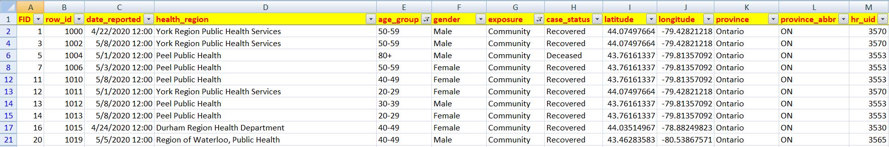
Today, I’ll be demonstrating some scenarios based on open-source data from Canada. In this post, I will only explain some of the significant parts of the code. Not the entire range of scripts here.
Let’s explore a couple of sample source data –
I would like to explore how much this disease caused an impact on the elderly in Canada.
Let’s explore the source directory structure –
For this, you need to install the following packages –
In this case, we’ve downloaded the data from Canada’s site. However, they have created API. So, you can consume the data through that way as well. Since the volume is a little large. I decided to download that in CSV & then use that for my analysis.
Before I start, let me explain a couple of critical assumptions that I had to make due to data impurities or availabilities.
If there is no data available for a specific case, my application will consider that patient as COVID-Active.
We will consider the patient is affected through Community-spreading until we have data to find it otherwise.
If there is no data available for gender, we’re marking these records as “Other.” So, that way, we’re making it into that category, where the patient doesn’t want to disclose their sexual orientation.
If we don’t have any data, then by default, the application is considering the patient is alive.
Lastly, my application considers the middle point of the age range data for all the categories, i.e., the patient’s age between 20 & 30 will be considered as 25.
1. clsCovidAnalysisByCountryAdv (This is the main script, which will invoke the Machine-Learning API & return 0 if successful.)
################################################## Written By: SATYAKI DE ######## Written On: 01-Jun-2020 ######## Modified On 01-Jun-2020 ######## ######## Objective: Main scripts for Logistic ######## Regression. ##################################################importpandasaspimportclsLaslogimportdatetimeimportmatplotlib.pyplotaspltimportseabornassnsfromclsConfigimport clsConfig as cf
# %matplotlib inline -- for Jupyter NotebookclassclsCovidAnalysisByCountryAdv:
def__init__(self):
self.fileName_1 = cf.config['FILE_NAME_1']
self.fileName_2 = cf.config['FILE_NAME_2']
self.Ind = cf.config['DEBUG_IND']
self.subdir =str(cf.config['LOG_DIR_NAME'])
defsetDefaultActiveCases(self, row):
try:
str_status =str(row['case_status'])
if str_status =='Not Reported':
return'Active'else:
return str_status
except:
return'Active'defsetDefaultExposure(self, row):
try:
str_exposure =str(row['exposure'])
if str_exposure =='Not Reported':
return'Community'else:
return str_exposure
except:
return'Community'defsetGender(self, row):
try:
str_gender =str(row['gender'])
if str_gender =='Not Reported':
return'Other'else:
return str_gender
except:
return'Other'defsetSurviveStatus(self, row):
try:
# 0 - Deceased# 1 - Alive
str_active =str(row['ActiveCases'])
if str_active =='Deceased':
return0else:
return1except:
return1defgetAgeFromGroup(self, row):
try:
# We'll take the middle of the Age group# If a age range falls with 20, we'll# consider this as 10.# Similarly, a age group between 20 & 30,# should reflect by 25.# Anything above 80 will be considered as# 85
str_age_group =str(row['AgeGroup'])
if str_age_group =='<20':
return10elif str_age_group =='20-29':
return25elif str_age_group =='30-39':
return35elif str_age_group =='40-49':
return45elif str_age_group =='50-59':
return55elif str_age_group =='60-69':
return65elif str_age_group =='70-79':
return75else:
return85except:
return100defpredictResult(self):
try:
# Initiating Logging Instances
clog = log.clsL()
# Important variables
var = datetime.datetime.now().strftime(".%H.%M.%S")
print('Target File Extension will contain the following:: ', var)
Ind =self.Ind
subdir =self.subdir
######################################## ## Using Logistic Regression to ## Idenitfy the following scenarios - ## ## Age wise Infection Vs Deaths ## ########################################
inputFileName_2 =self.fileName_2
# Reading from Input File
df_2 = p.read_csv(inputFileName_2)
# Fetching only relevant columns
df_2_Mod = df_2[['date_reported','age_group','gender','exposure','case_status']]
df_2_Mod['State'] = df_2['province_abbr']
print()
print('Projecting 2nd file sample rows: ')
print(df_2_Mod.head())
print()
x_row_1 = df_2_Mod.shape[0]
x_col_1 = df_2_Mod.shape[1]
print('Total Number of Rows: ', x_row_1)
print('Total Number of columns: ', x_col_1)
########################################################################################## Few Assumptions ########################################################################################### By default, if there is no data on exposure - We'll treat that as community spreading ## By default, if there is no data on case_status - We'll consider this as active ## By default, if there is no data on gender - We'll put that under a separate Gender ## category marked as the "Other". This includes someone who doesn't want to identify ## his/her gender or wants to be part of LGBT community in a generic term. ## ## We'll transform our data accordingly based on the above logic. ##########################################################################################
df_2_Mod['ActiveCases'] = df_2_Mod.apply(lambda row: self.setDefaultActiveCases(row), axis=1)
df_2_Mod['ExposureStatus'] = df_2_Mod.apply(lambda row: self.setDefaultExposure(row), axis=1)
df_2_Mod['Gender'] = df_2_Mod.apply(lambda row: self.setGender(row), axis=1)
# Filtering all other records where we don't get any relevant information# Fetching Data for
df_3 = df_2_Mod[(df_2_Mod['age_group'] !='Not Reported')]
# Dropping unwanted columns
df_3.drop(columns=['exposure'], inplace=True)
df_3.drop(columns=['case_status'], inplace=True)
df_3.drop(columns=['date_reported'], inplace=True)
df_3.drop(columns=['gender'], inplace=True)
# Renaming one existing column
df_3.rename(columns={"age_group": "AgeGroup"}, inplace=True)
# Creating important feature# 0 - Deceased# 1 - Alive
df_3['Survived'] = df_3.apply(lambda row: self.setSurviveStatus(row), axis=1)
clog.logr('2.df_3'+ var +'.csv', Ind, df_3, subdir)
print()
print('Projecting Filter sample rows: ')
print(df_3.head())
print()
x_row_2 = df_3.shape[0]
x_col_2 = df_3.shape[1]
print('Total Number of Rows: ', x_row_2)
print('Total Number of columns: ', x_col_2)
# Let's do some basic checkings
sns.set_style('whitegrid')
#sns.countplot(x='Survived', hue='Gender', data=df_3, palette='RdBu_r')# Fixing Gender Column# This will check & indicate yellow for missing entries#sns.heatmap(df_3.isnull(), yticklabels=False, cbar=False, cmap='viridis')#sex = p.get_dummies(df_3['Gender'], drop_first=True)
sex = p.get_dummies(df_3['Gender'])
df_4 = p.concat([df_3, sex], axis=1)
print('After New addition of columns: ')
print(df_4.head())
clog.logr('3.df_4'+ var +'.csv', Ind, df_4, subdir)
# Dropping unwanted columns for our Machine Learning
df_4.drop(columns=['Gender'], inplace=True)
df_4.drop(columns=['ActiveCases'], inplace=True)
df_4.drop(columns=['Male','Other','Transgender'], inplace=True)
clog.logr('4.df_4_Mod'+ var +'.csv', Ind, df_4, subdir)
# Fixing Spread Columns
spread = p.get_dummies(df_4['ExposureStatus'], drop_first=True)
df_5 = p.concat([df_4, spread], axis=1)
print('After Spread columns:')
print(df_5.head())
clog.logr('5.df_5'+ var +'.csv', Ind, df_5, subdir)
# Dropping unwanted columns for our Machine Learning
df_5.drop(columns=['ExposureStatus'], inplace=True)
clog.logr('6.df_5_Mod'+ var +'.csv', Ind, df_5, subdir)
# Fixing Age Columns
df_5['Age'] = df_5.apply(lambda row: self.getAgeFromGroup(row), axis=1)
df_5.drop(columns=["AgeGroup"], inplace=True)
clog.logr('7.df_6'+ var +'.csv', Ind, df_5, subdir)
# Fixing Dummy Columns Name# Renaming one existing column Travel-Related with Travel_Related
df_5.rename(columns={"Travel-Related": "TravelRelated"}, inplace=True)
clog.logr('8.df_7'+ var +'.csv', Ind, df_5, subdir)
# Removing state for temporary basis
df_5.drop(columns=['State'], inplace=True)
# df_5.drop(columns=['State','Other','Transgender','Pending','TravelRelated','Male'], inplace=True)# Casting this entire dataframe into Integer# df_5_temp.apply(p.to_numeric)print('Info::')
print(df_5.info())
print("*"*60)
print(df_5.describe())
print("*"*60)
clog.logr('9.df_8'+ var +'.csv', Ind, df_5, subdir)
print('Intermediate Sample Dataframe for Age::')
print(df_5.head())
# Plotting it to Graphsns.jointplot(x="Age", y='Survived', data=df_5)
sns.jointplot(x="Age", y='Survived', data=df_5, kind='kde', color='red')
plt.xlabel("Age")
plt.ylabel("Data Point (0 - Died Vs 1 - Alive)")# Another check with Age Group
sns.countplot(x='Survived', hue='Age', data=df_5, palette='RdBu_r')
plt.xlabel("Survived(0 - Died Vs 1 - Alive)")
plt.ylabel("Total No Of Patient")
df_6 = df_5.drop(columns=['Survived'], axis=1)
clog.logr('10.df_9'+ var +'.csv', Ind, df_6, subdir)
# Train & Split Data
x_1 = df_6
y_1 = df_5['Survived']
# Now Train-Test Split of your source datafromsklearn.model_selectionimport train_test_split
# test_size => % of allocated data for your test cases# random_state => A specific set of random split on your data
X_train_1, X_test_1, Y_train_1, Y_test_1 = train_test_split(x_1, y_1, test_size=0.3, random_state=101)
# Importing Modelfromsklearn.linear_modelimport LogisticRegression
logmodel = LogisticRegression()
logmodel.fit(X_train_1, Y_train_1)
# Adding Predictions to it
predictions_1 = logmodel.predict(X_test_1)
fromsklearn.metricsimport classification_report
print('Classification Report:: ')
print(classification_report(Y_test_1, predictions_1))
fromsklearn.metricsimport confusion_matrix
print('Confusion Matrix:: ')
print(confusion_matrix(Y_test_1, predictions_1))
# This is require when you are trying to print from conventional# front & not using Jupyter notebook.
plt.show()
return0exceptExceptionas e:
x =str(e)
print('Error : ', x)
return1
Key snippets from the above script –
df_2_Mod['ActiveCases'] = df_2_Mod.apply(lambda row: self.setDefaultActiveCases(row), axis=1)df_2_Mod['ExposureStatus'] = df_2_Mod.apply(lambda row: self.setDefaultExposure(row), axis=1)df_2_Mod['Gender'] = df_2_Mod.apply(lambda row: self.setGender(row), axis=1)# Filtering all other records where we don't get any relevant information# Fetching Data fordf_3 = df_2_Mod[(df_2_Mod['age_group'] != 'Not Reported')]# Dropping unwanted columnsdf_3.drop(columns=['exposure'], inplace=True)df_3.drop(columns=['case_status'], inplace=True)df_3.drop(columns=['date_reported'], inplace=True)df_3.drop(columns=['gender'], inplace=True)# Renaming one existing columndf_3.rename(columns={"age_group": "AgeGroup"}, inplace=True)# Creating important feature# 0 - Deceased# 1 - Alivedf_3['Survived'] = df_3.apply(lambda row: self.setSurviveStatus(row), axis=1)
The above lines point to the critical transformation areas, where the application is invoking various essential business logic.
The above lines will transform the data into this –
As you can see, we’ve transformed the row values into columns with binary values. This kind of transformation is beneficial.
# Plotting it to Graphsns.jointplot(x="Age", y='Survived', data=df_5)sns.jointplot(x="Age", y='Survived', data=df_5, kind='kde', color='red')plt.xlabel("Age")plt.ylabel("Data Point (0 - Died Vs 1 - Alive)")# Another check with Age Groupsns.countplot(x='Survived', hue='Age', data=df_5, palette='RdBu_r')plt.xlabel("Survived(0 - Died Vs 1 - Alive)")plt.ylabel("Total No Of Patient")
The above lines will process the data & visualize based on that.
x_1 = df_6y_1 = df_5['Survived']
In the above snippet, we’ve assigned the features & target variable for our final logistic regression model.
# Now Train-Test Split of your source datafrom sklearn.model_selection import train_test_split# test_size => % of allocated data for your test cases# random_state => A specific set of random split on your dataX_train_1, X_test_1, Y_train_1, Y_test_1 = train_test_split(x_1, y_1, test_size=0.3, random_state=101)# Importing Modelfrom sklearn.linear_model import LogisticRegressionlogmodel = LogisticRegression()logmodel.fit(X_train_1, Y_train_1)
In the above snippet, we’re splitting the primary data & create a set of test & train data. Once we have the collection, the application will put the logistic regression model. And, finally, we’ll fit the training data.
The above lines, finally use the model & then we feed our test data.
Let’s see how it runs –
And, here is the log directory –
For better understanding, I’m just clubbing both the diagram at one place & the final outcome is showing as follows –
So, from the above picture, we can see that the maximum vulnerable patients are patients who are 80+. The next two categories that also suffered are 70+ & 60+.
Also, We’ve checked the Female Vs. Male in the following code –
sns.countplot(x='Survived', hue='Female', data=df_5, palette='RdBu_r')plt.xlabel("Survived(0 - Died Vs 1 - Alive)")plt.ylabel("Female Vs Male (Including Other Genders)")
And, the analysis represents through this –
In this case, you have to consider that the Male part includes all the other genders apart from the actual Male. Hence, I believe death for females would be more compared to people who identified themselves as males.
So, finally, we’ve done it.
During this challenging time, I would request you to follow strict health guidelines & stay healthy.
N.B.: All the data that are used here can be found in the public domain. We use this solely for educational purposes. You can find the details here.
Today, I’ll be presenting a different kind of post here. I’ll be trying to predict health issues for senior citizens based on “realtime weather data” by blending open-source population data using some mock risk factor calculation. At the end of the post, I’ll be plotting these numbers into some graphs for better understanding.
Let’s drive!
For this first, we need realtime weather data. To do that, we need to subscribe to the data from OpenWeather API. For that, you have to register as a developer & you’ll receive a similar email from them once they have approved –
So, from the above picture, you can see that, you’ll be provided one API key & also offered a couple of useful API documentation. I would recommend exploring all the links before you try to use it.
You can also view your API key once you logged into their console. You can also create multiple API keys & the screen should look something like this –
For security reasons, I’ll be hiding my own keys & the same should be applicable for you as well.
I would say many of these free APIs might have some issues. So, I would recommend you to start testing the open API through postman before you jump into the Python development. Here is the glimpse of my test through the postman –
Once, I can see that the API is returning the result. I can work on it.
Apart from that, one needs to understand that these API might have limited use & also you need to know the consequences in terms of price & tier in case if you exceeded the limit. Here is the detail for this API –
For our demo, I’ll be using the Free tire only.
Let’s look into our other source data. We got the top 10 city population-wise over there internet. Also, we have collected sample Senior Citizen percentage against sex ratio across those cities. We have masked these values on top of that as this is just for education purposes.
1. CityDetails.csv
Here is the glimpse of this file –
So, this file only contains the total population across the top 10 cities in the USA.
2. SeniorCitizen.csv
This file contains the Sex ratio of Senior citizens across those top 10 cities by population.
Again, we are not going to discuss any script, which we’ve already discussed here.
Hence, we’re skipping clsL.py here.
1. clsConfig.py (This script contains all the parameters of the server.)
In the above snippet, our application first preparing the payload & the parameters received from our param script. And then invoke the GET method to extract the real-time data in the form of JSON & finally sending the JSON payload to the primary calling function.
3. clsMap.py (This script contains the main logic to prepare the MAP using seaborn package & try to plot our custom made risk factor by blending the realtime data with our statistical data received over the internet.)
################################################## Written By: SATYAKI DE ######## Written On: 19-Jan-2020 ######## Modified On 19-Jan-2020 ######## ######## Objective: Main scripts to invoke ######## plot into the Map. ##################################################importseabornassnsimportloggingfromclsConfigimport clsConfig as cf
importpandasaspimportclsLascl# This library requires later# to print the chartimportmatplotlib.pyplotaspltclassclsMap:
def__init__(self):
self.src_file = cf.config['SRC_FILE_1']
defcalculateRisk(self, row):
try:
# Let's assume some logic# 1. By default, 30% of Senior Citizen# prone to health Issue for each City# 2. Male Senior Citizen is 19% more prone# to illness than female.# 3. If humidity more than 70% or less# than 40% are 22% main cause of illness# 4. If feels like more than 280 or# less than 260 degree are 17% more prone# to illness.# Finally, this will be calculated per 1K# people around 10 blocks
str_sex =str(row['Sex'])
int_humidity =int(row['humidity'])
int_feelsLike =int(row['feels_like'])
int_population =int(str(row['Population']).replace(',',''))
float_srcitizen =float(row['SeniorCitizen'])
confidance_score =0.0
SeniorCitizenPopulation = (int_population * float_srcitizen)
if str_sex =='Male':
confidance_score = (SeniorCitizenPopulation *0.30*0.19) + confidance_score
else:
confidance_score = (SeniorCitizenPopulation *0.30*0.11) + confidance_score
if ((int_humidity >70) | (int_humidity <40)):
confidance_score = confidance_score + (int_population *0.30* float_srcitizen) *0.22if ((int_feelsLike >280) | (int_feelsLike <260)):
confidance_score = confidance_score + (int_population *0.30* float_srcitizen) *0.17
final_score =round(round(confidance_score, 2) / (1000*10), 2)
return final_score
exceptExceptionas e:
x =str(e)
return x
defsetMap(self, dfInput):
try:
resVal =0
df = p.DataFrame()
debug_ind ='Y'
src_file =self.src_file
# Initiating Log Class
l = cl.clsL()
df = dfInput
# Creating a subset of desired columns
dfMod = df[['CityName', 'temp', 'Population', 'humidity', 'feels_like']]

l.logr('5.dfSuppliment.csv', debug_ind, dfMod, 'log')

# Fetching Senior Citizen Data
df = p.read_csv(src_file, index_col=False)

# Merging two frames
dfMerge = p.merge(df, dfMod, on=['CityName'])

l.logr('6.dfMerge.csv', debug_ind, dfMerge, 'log')

# Getting RiskFactor quotient from our custom made logic
dfMerge['RiskFactor'] = dfMerge.apply(lambda row: self.calculateRisk(row), axis=1)

l.logr('7.dfRiskFactor.csv', debug_ind, dfMerge, 'log')
# Generating Map plotss# sns.lmplot(x='RiskFactor', y='SeniorCitizen', data=dfMerge, hue='Sex')# sns.lmplot(x='RiskFactor', y='SeniorCitizen', data=dfMerge, hue='Sex', markers=['o','v'], scatter_kws={'s':25})
sns.lmplot(x='RiskFactor', y='SeniorCitizen', data=dfMerge, col='Sex')
# This is required when you are running# through normal Python & not through# Jupyter Notebook
plt.show()
return resVal
exceptExceptionas e:
x =str(e)
print(x)
logging.info(x)
resVal = x
return resVal
Key lines from the above codebase –
# Creating a subset of desired columnsdfMod = df[['CityName', 'temp', 'Population', 'humidity', 'feels_like']]l.logr('5.dfSuppliment.csv', debug_ind, dfMod, 'log')# Fetching Senior Citizen Datadf = p.read_csv(src_file, index_col=False)# Merging two framesdfMerge = p.merge(df, dfMod, on=['CityName'])l.logr('6.dfMerge.csv', debug_ind, dfMerge, 'log')# Getting RiskFactor quotient from our custom made logicdfMerge['RiskFactor'] = dfMerge.apply(lambda row: self.calculateRisk(row), axis=1)l.logr('7.dfRiskFactor.csv', debug_ind, dfMerge, 'log')
Combining our Senior Citizen data with already processed data coming from our primary calling script. Also, here the application is calculating our custom logic to find out the risk factor figures. If you want to go through that, I’ve provided the logic to derive it. However, this is just a demo to find out similar figures. You should not rely on the logic that I’ve used (It is kind of my observation of life till now. :D).
The below lines are only required when you are running seaborn, not via Jupyter notebook.
plt.show()
4. callOpenMapWeatherAPI.py (This is the first calling script. This script also calls the realtime API & then blend the first file with it & pass the only relevant columns of data to our Map script to produce the graph.)
################################################## Written By: SATYAKI DE ######## Written On: 19-Jan-2020 ######## Modified On 19-Jan-2020 ######## ######## Objective: Main calling scripts. ##################################################fromclsConfigimport clsConfig as cf
importpandasaspimportclsLasclimportloggingimportdatetimeimportjsonimportclsWeatherasctimportreimportnumpyasnpimportclsMapascm# Disbling Warningdefwarn(*args, **kwargs):
passimportwarnings
warnings.warn = warn
# Lookup functions from# Azure cloud SQL DB
var = datetime.datetime.now().strftime("%Y-%m-%d_%H-%M-%S")
defgetMainWeather(row):
try:
# Using regular expression to fetch time part only
lkp_Columns =str(row['weather'])
jpayload =str(lkp_Columns).replace("'", '"')
#jpayload = json.dumps(lkp_Columns)
payload = json.loads(jpayload)
df_lkp = p.io.json.json_normalize(payload)
df_lkp.columns = df_lkp.columns.map(lambda x: x.split(".")[-1])
str_main_weather =str(df_lkp.iloc[0]['main'])
return str_main_weather
exceptExceptionas e:
x =str(e)
str_main_weather = x
return str_main_weather
defgetMainDescription(row):
try:
# Using regular expression to fetch time part only
lkp_Columns =str(row['weather'])
jpayload =str(lkp_Columns).replace("'", '"')
#jpayload = json.dumps(lkp_Columns)
payload = json.loads(jpayload)
df_lkp = p.io.json.json_normalize(payload)
df_lkp.columns = df_lkp.columns.map(lambda x: x.split(".")[-1])
str_description =str(df_lkp.iloc[0]['description'])
return str_description
exceptExceptionas e:
x =str(e)
str_description = x
return str_description
defmain():
try:
dfSrc = p.DataFrame()
df_ret = p.DataFrame()
ret_2 =''
debug_ind ='Y'
general_log_path =str(cf.config['LOG_PATH'])
# Enabling Logging Info
logging.basicConfig(filename=general_log_path +'consolidatedIR.log', level=logging.INFO)
# Initiating Log Class
l = cl.clsL()
# Moving previous day log files to archive directory
arch_dir = cf.config['ARCH_DIR']
log_dir = cf.config['LOG_PATH']
col_list = cf.config['COL_LIST']
col_list_1 = cf.config['COL_LIST_1']
col_list_2 = cf.config['COL_LIST_2']
tmpR0 ="*"*157
logging.info(tmpR0)
tmpR9 ='Start Time: '+str(var)
logging.info(tmpR9)
logging.info(tmpR0)
print("Archive Directory:: ", arch_dir)
print("Log Directory::", log_dir)
tmpR1 ='Log Directory::'+ log_dir
logging.info(tmpR1)
df2 = p.DataFrame()
src_file = cf.config['SRC_FILE']
# Fetching data from source file
df = p.read_csv(src_file, index_col=False)
# Creating a list of City Name from the source file
city_list = df['CityName'].tolist()
# Declaring an empty dictionary
merge_dict = {}
merge_dict['city'] = df2
start_pos =1
src_file_name ='1.'+ cf.config['SRC_FILE_INIT']
for i in city_list:
x1 = ct.clsWeather()
ret_2 = x1.searchQry(i)
# Capturing the JSON Payload
res = json.loads(ret_2)
# Converting dictionary to Pandas Dataframe# df_ret = p.read_json(ret_2, orient='records')
df_ret = p.io.json.json_normalize(res)
df_ret.columns = df_ret.columns.map(lambda x: x.split(".")[-1])
# Removing any duplicate columns
df_ret = df_ret.loc[:, ~df_ret.columns.duplicated()]
# l.logr(str(start_pos) + '.1.' + src_file_name, debug_ind, df_ret, 'log')
start_pos = start_pos +1# If all the conversion successful# you won't get any gust column# from OpenMap response. Hence, we# need to add dummy reason column# to maintain the consistent structuresif'gust'notin df_ret.columns:
df_ret = df_ret.assign(gust=999999)[['gust'] + df_ret.columns.tolist()]
# Resetting the column orders as per JSON
column_order = col_list
df_mod_ret = df_ret.reindex(column_order, axis=1)
if start_pos ==1:
merge_dict['city'] = df_mod_ret
else:
d_frames = [merge_dict['city'], df_mod_ret]
merge_dict['city'] = p.concat(d_frames)
start_pos +=1for k, v in merge_dict.items():
l.logr(src_file_name, debug_ind, merge_dict[k], 'log')
# Now opening the temporary file
temp_log_file = log_dir + src_file_name
dfNew = p.read_csv(temp_log_file, index_col=False)
# Extracting Complex columns
dfNew['WeatherMain'] = dfNew.apply(lambda row: getMainWeather(row), axis=1)
dfNew['WeatherDescription'] = dfNew.apply(lambda row: getMainDescription(row), axis=1)
l.logr('2.dfNew.csv', debug_ind, dfNew, 'log')
# Removing unwanted columns & Renaming key columns
dfNew.drop(['weather'], axis=1, inplace=True)
dfNew.rename(columns={'name': 'CityName'}, inplace=True)
l.logr('3.dfNewMod.csv', debug_ind, dfNew, 'log')
# Now joining with the main csv# to get the complete picture
dfMain = p.merge(df, dfNew, on=['CityName'])
l.logr('4.dfMain.csv', debug_ind, dfMain, 'log')
# Let's extract only relevant columns
dfSuppliment = dfMain[['CityName', 'Population', 'State', 'country', 'feels_like', 'humidity', 'pressure', 'temp', 'temp_max', 'temp_min', 'visibility', 'deg', 'gust', 'speed', 'WeatherMain', 'WeatherDescription']]
l.logr('5.dfSuppliment.csv', debug_ind, dfSuppliment, 'log')
# Let's pass this to our map section
x2 = cm.clsMap()
ret_3 = x2.setMap(dfSuppliment)
if ret_3 ==0:
print('Successful Map Generated!')
else:
print('Please check the log for further issue!')
print("-"*60)
print()
print('Finding Story points..')
print("*"*157)
logging.info('Finding Story points..')
logging.info(tmpR0)
tmpR10 ='End Time: '+str(var)
logging.info(tmpR10)
logging.info(tmpR0)
exceptValueErroras e:
print(str(e))
print("No relevant data to proceed!")
logging.info("No relevant data to proceed!")
exceptExceptionas e:
print("Top level Error: args:{0}, message{1}".format(e.args, e.message))
if __name__ =="__main__":
main()
Key snippet from the above script –
# Capturing the JSON Payloadres = json.loads(ret_2)# Converting dictionary to Pandas Dataframedf_ret = p.io.json.json_normalize(res)df_ret.columns = df_ret.columns.map(lambda x: x.split(".")[-1])
Once the application received the JSON response from the realtime API, the application is converting it to pandas dataframe.
# Removing any duplicate columnsdf_ret = df_ret.loc[:, ~df_ret.columns.duplicated()]
Since this is a complex JSON response. The application might encounter duplicate columns, which might cause a problem later. Hence, our app is removing all these duplicate columns as they are not required for our cases.
if 'gust' not in df_ret.columns:
    df_ret = df_ret.assign(gust=999999)[['gust'] + df_ret.columns.tolist()]
There is a possibility that the application might not receive all the desired attributes from the realtime API. Hence, the above lines will check & add a dummy column named gust for those records in case if they are not present in the JSON response.
These few lines required as our API has a limitation of responding with only one city at a time. Hence, in this case, we’re retrieving one town at a time & finally merge them into a single dataframe before creating a temporary source file for the next step.
At this moment our data should look like this –
Let’s check the weather column. We need to extract the main & description for our dashboard, which will be coming in the next installment.
The above lines extracting the weather column & replacing the single quotes with the double quotes before the application is trying to convert that to JSON. Once it converted to JSON, the json_normalize will easily serialize it & create individual columns out of it. Once you have them captured inside the pandas dataframe, you can extract the unique values & store them & return them to your primary calling function.
# Let's pass this to our map sectionx2 = cm.clsMap()ret_3 = x2.setMap(dfSuppliment)if ret_3 == 0: print('Successful Map Generated!')else: print('Please check the log for further issue!')
In the above lines, the application will invoke the Map class to calculate the remaining logic & then plotting the data into the seaborn graph.
Let’s just briefly see the central directory structure –
Here is the log directory –
And, finally, the source directory should look something like this –
Here is the post as to how to call this Dnpr library & what are the current limitations of this library.
Before we start let’s post the calling script & then explain how we can use them –
##############################################
#### Written By: SATYAKI DE ####
#### Written On: 08-Sep-2019 ####
#### ####
#### Objective: Main calling scripts. ####
##############################################
from dnpr.clsDnpr import clsDnpr
import datetime as dt
import json
# Disbling Warning
def warn(*args, **kwargs):
pass
import warnings
warnings.warn = warn
# Lookup functions from
def main():
try:
srcJson = [
            {"FirstName": "Satyaki", "LastName": "De", "Sal": 1000},
            {"FirstName": "Satyaki", "LastName": "De", "Sal": 1000},
            {"FirstName": "Archi", "LastName": "Bose", "Sal": 500},
            {"FirstName": "Archi", "LastName": "Bose", "Sal": 7000},
            {"FirstName": "Deb", "LastName": "Sen", "Sal": 9500}
          ]
print("=" * 157)
print("Checking distinct function!")
print("=" * 157)
print()
print("*" * 157)
print("Input Data: ")
srcJsonFormat = json.dumps(srcJson, indent=1)
print(str(srcJsonFormat))
print("*" * 157)
# Initializing the class
t = clsDnpr()
print("1. Checking distinct functionality!")
var1 = dt.datetime.now().strftime("%Y-%m-%d %H-%M-%S")
print("Start Time: ", str(var1))
# Invoking the distinct function
tarJson = t.distinct(srcJson)
print("*" * 157)
print("Output Data: ")
tarJsonFormat = json.dumps(tarJson, indent=1)
print(str(tarJsonFormat))
print("*" * 157)
if not tarJson:
print()
print("No relevant output data!")
print("*" * 157)
else:
print()
print("Relevant output data comes!")
print("*" * 157)
var2 = dt.datetime.now().strftime("%Y-%m-%d %H-%M-%S")
print("End Time: ", str(var2))
print("=" * 157)
print("End of distinct function!")
print("=" * 157)
print("2. Checking nvl functionality!")
srcJson_1 = [
{"FirstName": "Satyaki", "LastName": "", "Sal": 1000},
{"FirstName": "Archi", "LastName": "Bose", "Sal": 500},
{"FirstName": "Deb", "LastName": "", "Sal": 9500}
]
var3 = dt.datetime.now().strftime("%Y-%m-%d %H-%M-%S")
print("Start Time: ", str(var3))
strDef = 'FNU'
print("Default Value: ", strDef)
srcColName = 'LastName'
print('Candidate Column for NVL: ', srcColName)
# Invoking the nvl function
tarJson_1 = t.nvl(srcJson_1, srcColName, strDef)
print("*" * 157)
print("Output Data: ")
tarJsonFormat_1 = json.dumps(tarJson_1, indent=1)
print(str(tarJsonFormat_1))
print("*" * 157)
if not tarJson_1:
print()
print("No relevant output data!")
print("*" * 157)
else:
print()
print("Relevant output data comes!")
print("*" * 157)
var4 = dt.datetime.now().strftime("%Y-%m-%d %H-%M-%S")
print("End Time: ", str(var4))
print("=" * 157)
print("End of nvl function!")
print("=" * 157)
print("3. Checking partition-by functionality!")
srcJson_2 = [
{"FirstName": "Satyaki", "LastName": "", "Sal": 1000},
{"FirstName": "Satyaki", "LastName": "", "Sal": 700},
{"FirstName": "Archi", "LastName": "Bose", "Sal": 500},
{"FirstName": "Deb", "LastName": "", "Sal": 9500},
{"FirstName": "Archi", "LastName": "Bose", "Sal": 4500},
]
var5 = dt.datetime.now().strftime("%Y-%m-%d %H-%M-%S")
print("Start Time: ", str(var5))
GrList = ['FirstName', 'LastName']
print("Partition By Columns::: ", str(GrList))
grOperation = 'Max'
print('Operation toe be performed: ', grOperation)
strCandidateColumnName = 'Sal'
print('Column Name on which the aggregate function will take place: ', strCandidateColumnName)
# Invoking the partition by function - MAX
tarJson_1 = t.partitionBy(srcJson_2, GrList, grOperation, strCandidateColumnName)
print("*" * 157)
print("Output Data: ")
tarJsonFormat_1 = json.dumps(tarJson_1, indent=1)
print(str(tarJsonFormat_1))
print("*" * 157)
if not tarJson_1:
print()
print("No relevant output data!")
print("*" * 157)
else:
print()
print("Relevant output data comes!")
print("*" * 157)
var6 = dt.datetime.now().strftime("%Y-%m-%d %H-%M-%S")
print("End Time: ", str(var6))
var7 = dt.datetime.now().strftime("%Y-%m-%d %H-%M-%S")
print("Start Time: ", str(var7))
grOperation_1 = 'Min'
print('Operation toe be performed: ', grOperation_1)
# Invoking the Partition By function - MIN
tarJson_2 = t.partitionBy(srcJson_2, GrList, grOperation_1, strCandidateColumnName)
print("*" * 157)
print("Output Data: ")
tarJsonFormat_2 = json.dumps(tarJson_2, indent=1)
print(str(tarJsonFormat_2))
print("*" * 157)
if not tarJson_2:
print()
print("No relevant output data!")
print("*" * 157)
else:
print()
print("Relevant output data comes!")
print("*" * 157)
var8 = dt.datetime.now().strftime("%Y-%m-%d %H-%M-%S")
print("End Time: ", str(var8))
var9 = dt.datetime.now().strftime("%Y-%m-%d %H-%M-%S")
print("Start Time: ", str(var9))
grOperation_2 = 'Avg'
print('Operation toe be performed: ', grOperation_2)
# Invoking the Partition By function - Avg
tarJson_3 = t.partitionBy(srcJson_2, GrList, grOperation_2, strCandidateColumnName)
print("*" * 157)
print("Output Data: ")
tarJsonFormat_3 = json.dumps(tarJson_3, indent=1)
print(str(tarJsonFormat_3))
print("*" * 157)
if not tarJson_3:
print()
print("No relevant output data!")
print("*" * 157)
else:
print()
print("Relevant output data comes!")
print("*" * 157)
var10 = dt.datetime.now().strftime("%Y-%m-%d %H-%M-%S")
print("End Time: ", str(var10))
var11 = dt.datetime.now().strftime("%Y-%m-%d %H-%M-%S")
print("Start Time: ", str(var11))
grOperation_3 = 'Sum'
print('Operation toe be performed: ', grOperation_3)
# Invoking the Partition By function - Sum
tarJson_4 = t.partitionBy(srcJson_2, GrList, grOperation_3, strCandidateColumnName)
print("*" * 157)
print("Output Data: ")
tarJsonFormat_4 = json.dumps(tarJson_4, indent=1)
print(str(tarJsonFormat_4))
print("*" * 157)
if not tarJson_4:
print()
print("No relevant output data!")
print("*" * 157)
else:
print()
print("Relevant output data comes!")
print("*" * 157)
var12 = dt.datetime.now().strftime("%Y-%m-%d %H-%M-%S")
print("End Time: ", str(var12))
print("=" * 157)
print("End of partition function!")
print("=" * 157)
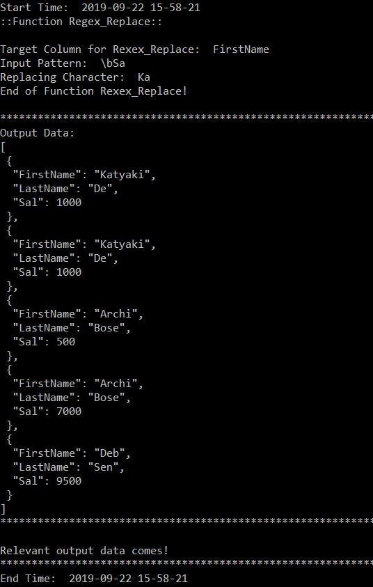
print("4. Checking regular expression functionality!")
print()
var13 = dt.datetime.now().strftime("%Y-%m-%d %H-%M-%S")
print("Start Time: ", str(var13))
print('::Function Regex_Like:: ')
print()
tarColumn = 'FirstName'
print('Target Column for Rexex_Like: ', tarColumn)
inpPattern = r"\bSa"
print('Input Pattern: ', str(inpPattern))
# Invoking the regex_like function
tarJson = t.regex_like(srcJson, tarColumn, inpPattern)
print('End of Function Regex_Like!')
print()
print("*" * 157)
print("Output Data: ")
tarJsonFormat = json.dumps(tarJson, indent=1)
print(str(tarJsonFormat))
print("*" * 157)
if not tarJson:
print()
print("No relevant output data!")
print("*" * 157)
else:
print()
print("Relevant output data comes!")
print("*" * 157)
var14 = dt.datetime.now().strftime("%Y-%m-%d %H-%M-%S")
print("End Time: ", str(var14))
var15 = dt.datetime.now().strftime("%Y-%m-%d %H-%M-%S")
print("Start Time: ", str(var15))
print('::Function Regex_Replace:: ')
print()
tarColumn = 'FirstName'
print('Target Column for Rexex_Replace: ', tarColumn)
inpPattern = r"\bSa"
print('Input Pattern: ', str(inpPattern))
replaceString = 'Ka'
print('Replacing Character: ', replaceString)
# Invoking the regex_replace function
tarJson = t.regex_replace(srcJson, tarColumn, inpPattern, replaceString)
print('End of Function Rexex_Replace!')
print()
print("*" * 157)
print("Output Data: ")
tarJsonFormat = json.dumps(tarJson, indent=1)
print(str(tarJsonFormat))
print("*" * 157)
if not tarJson:
print()
print("No relevant output data!")
print("*" * 157)
else:
print()
print("Relevant output data comes!")
print("*" * 157)
var16 = dt.datetime.now().strftime("%Y-%m-%d %H-%M-%S")
print("End Time: ", str(var16))
var17 = dt.datetime.now().strftime("%Y-%m-%d %H-%M-%S")
print("Start Time: ", str(var17))
print('::Function Regex_Substr:: ')
print()
tarColumn = 'FirstName'
print('Target Column for Regex_Substr: ', tarColumn)
inpPattern = r"\bSa"
print('Input Pattern: ', str(inpPattern))
# Invoking the regex_substr function
tarJson = t.regex_substr(srcJson, tarColumn, inpPattern)
print('End of Function Regex_Substr!')
print()
print("*" * 157)
print("Output Data: ")
tarJsonFormat = json.dumps(tarJson, indent=1)
print(str(tarJsonFormat))
print("*" * 157)
if not tarJson:
print()
print("No relevant output data!")
print("*" * 157)
else:
print()
print("Relevant output data comes!")
print("*" * 157)
var18 = dt.datetime.now().strftime("%Y-%m-%d %H-%M-%S")
print("End Time: ", str(var18))
print("=" * 157)
print("End of regular expression function!")
print("=" * 157)
except ValueError:
print("No relevant data to proceed!")
except Exception as e:
print("Top level Error: args:{0}, message{1}".format(e.args, e.message))
if __name__ == "__main__":
main()
Let’s explain the key lines –
As of now, the source payload that it will support is mostly simple JSON.
As you can see, we’ve relatively started with the simple JSON containing an array of elements.
# Initializing the class
t = clsDnpr()
In this line, you can initiate the main library.
Let’s explore the different functions, which you can use on JSON.
1. Distinct:
Let’s discuss the distinct function on JSON. This function can be extremely useful if you use NoSQL, which doesn’t offer any distinct features. Or, if you are dealing with or expecting your source with duplicate JSON inputs.
Let’s check our sample payload for distinct –
Here is the basic syntax & argument that it is expecting –
distinct(Input Json) returnOutput Json
So, all you have to ensure that you are passing a JSON input string.
As per our example –
# Invoking the distinct function tarJson = t.distinct(srcJson)
And, here is the output –
If you compare the source JSON. You would have noticed that there are two identical entries with the name “Satyaki” is now replaced by one unique entries.
Limitation: Currently, this will support only basic JSON. However, I’m working on it to support that much more complex hierarchical JSON in coming days.
2. NVL:
NVL is another feature that I guess platform like JSON should have. So, I built this library specially handles the NULL data scenario, where the developer may want to pass a default value in place of NULL.
Hence, the implementation of this function.
Here is the sample payload for this –
In this case, if there is some business logic that requires null values replaced with some default value for LastName say e.g. FNU. This function will help you to implement that logic.
Here is the basic syntax & argument that it is expecting –
nvl(
     Input Json,
     Prospective Null Column Name,
     Dafult Value in case of Null
   ) return Output Json
# Invoking the nvl function tarJson_1 = t.nvl(srcJson_1, srcColName, strDef)
So, in the above lines, this code will replace the Null value with the “FNU” for the column LastName.
And, Here is the output –
3. Partition_By:
I personally like this function as this gives more power to manipulate any data in JSON levels such as Avg, Min, Max or Sum. This might be very useful in order to implement some basic aggregation on the fly.
Here is the basic syntax & argument that it is expecting –
partition_by(
              Input Json,
              Group By Column List,
              Group By Operation,
              Candidate Column Name,
              Output Column Name
            ) return Output Json
Now, we would explore the sample payload for all these functions to test –
Case 1:
In this case, we’ll calculate the maximum salary against FirstName & LastName. However, I want to print the Location in my final JSON output.
So, if you see the sample data & let’s make it tabular for better understanding –
So, as per our business logic, our MAX aggregate would operate only on FirstName & LastName. Hence, the calculation will process accordingly.
In that case, the output will look something like –
As you can see, from the above picture two things happen. It will remove any duplicate entries. In this case, Satyaki has exactly two identical rows. So, it removes one. However, as part of partition by clause, it keeps two entries of Archi as the location is different. Deb will be appearing once as expected.
Let’s run our application & find out the output –
So, we meet our expectation.
Case 2:
Same, logic will be applicable for Min as well.
Hence, as per the table, we should expect the output as –
And, the output of our application run is –
So, this also come as expected.
Case 3:
Let’s check for average –
The only thing I wanted to point out, as we’ve two separate entries for Satyaki. So, the average will contain the salary from both the value as rightfully so. Hence, the average of (1000+700)/2 = 850.
Let’s run our application –
So, we’ve achieved our target.
Case 4:
Let’s check for Sum.
Now, let’s run our application –
In the next installment, we’ll be discussing the last function from this package i.e. Regular Expression in JSON.
I hope, you’ll like this presentation.
Let me know – if you find any special bug. I’ll look into that.
Till then – Happy Avenging!
Note: All the data posted here are representational data & available over the internet & for educational purpose only.
Please find the link of the PyPI package of new enhanced JSON library on Python. This is particularly very useful as I’ve accommodated the following features into it.
distinct
nvl
partition_by
regex_like
regex_replace
regex_substr
All these functions can be used over JSON payload through python. I’ll discuss this in details in my next blog post.
However, I would like to suggest this library that will be handy for NoSQL databases like Cosmos DB. Now, you can quickly implement many of these features such as distinct, partitioning & regular expressions with less effort.
Friends, this page mainly deals with the basic of oracle sql & pl/sql. Here, i’m going to present many useful Oracle snippets which can be plugged into your solution. Many of the snippets which are going to be part of this blog are conceptualize and coded by me and many cases i got the idea from our brilliant otn members. I’m sure you people will like all the snippets as useful bricks. Very soon i am going to post many oracle sql & pl/sql .
Here i’m posting some useful SQL snippets which can be plugged into your environment –
SQL:
1. Dynamic Table Alteration:Here is the sample code that demonstrate this –
scott>select * from v$version; BANNER ---------------------------------------------------------------- Oracle Database 10g Enterprise Edition Release 10.2.0.3.0 - Prod PL/SQL Release 10.2.0.3.0 - Production CORE 10.2.0.3.0 Production TNS for 32-bit Windows: Version 10.2.0.3.0 - Production NLSRTL Version 10.2.0.3.0 - Production
Elapsed: 00:00:05.00 scott> scott> scott>alter table &tab add (& col varchar2 ( 10 )); Enter value for tab: test_dummy Enter value for col: b old 1: alter table &tab add (& col varchar2 ( 10 )) new 1: alter table test_dummy add (b varchar2 ( 10 ))
Table altered.
Elapsed: 00:00:01.19
scott> scott>desc test_dummy; Name Null? Type -------------------- -------- -------------- A VARCHAR2(10) B VARCHAR2(10)
2. Alternative Of Break Command:
scott>
scott>SELECT lag(null, 1, d.dname)
over (partition by e.deptno order by e.ename) as dname,
2         e.ename
3  from emp e, dept d
4  where e.deptno = d.deptno
5  ORDER BY D.dname, e.ename;

DNAME          ENAME
-------------- ----------
ACCOUNTING     CLARK
KING
MILLER
RESEARCH       ADAMS
FORD
JONES
SCOTT
SMITH
SALES          ALLEN
BLAKE
JAMES

DNAME          ENAME
-------------- ----------
MARTIN
TURNER
WARD

14 rows selected.

Elapsed: 00:00:00.52
scott>
3. Can we increase the size of a column for a View:
SQL> create or replace view v_emp
2 as
3 select ename
4 from emp
5 /
View created.

SQL> desc v_emp
Name Null? Type
----------------------------------------- -------- ----------------------------
ENAME VARCHAR2(10)
SQL>
SQL> create or replace view v_emp
2 as
3 select cast (ename as varchar2 (30)) ename
4 from emp
5 /
View created.

SQL> desc v_emp
Name Null? Type
----------------------------------------- -------- ----------------------------
ENAME VARCHAR2(30)
And here is the silly way to do this –
create or replace view temp_vv
as
select replace(ename,' ') ename
from (
select rpad(ename,100) ename
from emp
);
4. Combining two SQL Into One:
satyaki> satyaki>select e.empno,e.deptno,d.loc "DEPT_10" 2 from emp e, dept d 3 where e.deptno = d.deptno 4 and d.deptno = 10;
EMPNO DEPTNO DEPT_10 ---------- ---------- ------------- 7782 10 NEW YORK 7839 10 NEW YORK 7934 10 NEW YORK
Elapsed: 00:00:00.04 satyaki> satyaki>select e.empno,e.deptno,d.loc "DEPT_OTH" 2 from emp e, dept d 3 where e.deptno = d.deptno 4 and e.deptno not in (10);
EMPNO DEPTNO DEPT_OTH ---------- ---------- ------------- 7369 20 DALLAS 7876 20 DALLAS 7566 20 DALLAS 7788 20 DALLAS 7902 20 DALLAS 7900 30 CHICAGO 7844 30 CHICAGO 7654 30 CHICAGO 7521 30 CHICAGO 7499 30 CHICAGO 7698 30 CHICAGO
11 rows selected.
Elapsed: 00:00:00.04 satyaki> satyaki> satyaki>select a.empno,( 2 select d.loc 3 from emp e, dept d 4 where e.deptno = d.deptno 5 and e.empno = a.empno 6 and d.deptno = 10 7 ) "DEPT_10" , 8 ( 9 select d.loc 10 from emp e, dept d 11 where e.deptno = d.deptno 12 and e.empno = a.empno 13 and d.deptno not in (10) 14 ) "DEPT_OTH" 15 from emp a 16 order by a.empno;
EMPNO DEPT_10 DEPT_OTH ---------- ------------- ------------- 7369 DALLAS 7499 CHICAGO 7521 CHICAGO 7566 DALLAS 7654 CHICAGO 7698 CHICAGO 7782 NEW YORK 7788 DALLAS 7839 NEW YORK 7844 CHICAGO 7876 DALLAS
EMPNO DEPT_10 DEPT_OTH ---------- ------------- ------------- 7900 CHICAGO 7902 DALLAS 7934 NEW YORK


You must be logged in to post a comment.