
Today, I’ll be sharing one of the most exciting posts I’ve ever shared. This post is rare as you cannot find the most relevant working solution easily over the net.
So, what are we talking about here? We’re going to build a Python-based iOS App using the Kivy framework. You get plenty of videos & documents on this as well. However, nowhere you’ll find the capability that I’m about to disclose. We’ll consume live IoT streaming data from a dummy application & then plot them in a MatplotLib dashboard inside the mobile App. And that’s where this post is seriously different from the rest of the available white papers.
But, before we dig into more details, let us see a quick demo of our iOS App.
Demo:

Isn’t it exciting? Great! Now, let’s dig into the details.
Let’s understand the architecture as to how we want to proceed with the solution here.
Architecture:

The above diagram shows that the Kive-based iOS application that will consume streaming data from the Ably queue. The initial dummy IoT application will push the real-time events to the same Ably queue.
So, now we understand the architecture. Fantastic!
Let’s deep dive into the code that we specifically built for this use case.
Code:
- IoTDataGen.py (Publishing Streaming data to Ably channels & captured IoT events from the simulator & publish them in Dashboard through measured KPIs.)
This file contains hidden or bidirectional Unicode text that may be interpreted or compiled differently than what appears below. To review, open the file in an editor that reveals hidden Unicode characters.
Learn more about bidirectional Unicode characters
| ############################################## | |
| #### Updated By: SATYAKI DE #### | |
| #### Updated On: 12-Nov-2021 #### | |
| #### #### | |
| #### Objective: Publishing Streaming data #### | |
| #### to Ably channels & captured IoT #### | |
| #### events from the simulator & publish #### | |
| #### them in Dashboard through measured #### | |
| #### KPIs. #### | |
| #### #### | |
| ############################################## | |
| import random | |
| import time | |
| import json | |
| import clsPublishStream as cps | |
| import datetime | |
| from clsConfig import clsConfig as cf | |
| import logging | |
| # Invoking the IoT Device Generator. | |
| def main(): | |
| ############################################### | |
| ### Global Section ### | |
| ############################################### | |
| # Initiating Ably class to push events | |
| x1 = cps.clsPublishStream() | |
| ############################################### | |
| ### End of Global Section ### | |
| ############################################### | |
| # Initiating Log Class | |
| general_log_path = str(cf.conf['LOG_PATH']) | |
| msgSize = int(cf.conf['limRec']) | |
| # Enabling Logging Info | |
| logging.basicConfig(filename=general_log_path + 'IoTDevice.log', level=logging.INFO) | |
| # Other useful variables | |
| cnt = 1 | |
| idx = 0 | |
| debugInd = 'Y' | |
| x_value = 0 | |
| total_1 = 100 | |
| total_2 = 100 | |
| var = datetime.datetime.now().strftime("%Y-%m-%d_%H-%M-%S") | |
| # End of usefull variables | |
| while True: | |
| srcJson = { | |
| "x_value": x_value, | |
| "total_1": total_1, | |
| "total_2": total_2 | |
| } | |
| x_value += 1 | |
| total_1 = total_1 + random.randint(-6, 8) | |
| total_2 = total_2 + random.randint(-5, 6) | |
| tmpJson = str(srcJson) | |
| if cnt == 1: | |
| srcJsonMast = '{' + '"' + str(idx) + '":'+ tmpJson | |
| elif cnt == msgSize: | |
| srcJsonMast = srcJsonMast + '}' | |
| print('JSON: ') | |
| print(str(srcJsonMast)) | |
| # Pushing both the Historical Confirmed Cases | |
| retVal_1 = x1.pushEvents(srcJsonMast, debugInd, var) | |
| if retVal_1 == 0: | |
| print('Successfully IoT event pushed!') | |
| else: | |
| print('Failed to push IoT events!') | |
| srcJsonMast = '' | |
| tmpJson = '' | |
| cnt = 0 | |
| idx = -1 | |
| srcJson = {} | |
| retVal_1 = 0 | |
| else: | |
| srcJsonMast = srcJsonMast + ',' + '"' + str(idx) + '":'+ tmpJson | |
| cnt += 1 | |
| idx += 1 | |
| time.sleep(1) | |
| if __name__ == "__main__": | |
| main() |
Let’s explore the key snippets from the above script.
# Initiating Ably class to push events
x1 = cps.clsPublishStream()
The I-OS App is calling the main class to publish the JSON events to Ably Queue.
if cnt == 1:
    srcJsonMast = '{' + '"' + str(idx) + '":'+ tmpJson
elif cnt == msgSize:
    srcJsonMast = srcJsonMast + '}'
    print('JSON: ')
    print(str(srcJsonMast))

    # Pushing both the Historical Confirmed Cases
    retVal_1 = x1.pushEvents(srcJsonMast, debugInd, var)

    if retVal_1 == 0:
        print('Successfully IoT event pushed!')
    else:
        print('Failed to push IoT events!')

    srcJsonMast = ''
    tmpJson = ''
    cnt = 0
    idx = -1
    srcJson = {}
    retVal_1 = 0
else:
    srcJsonMast = srcJsonMast + ',' + '"' + str(idx) + '":'+ tmpJson
In the above snippet, we’re forming the payload dynamically & then calling the “pushEvents” to push all the random generated IoT mock-events to the Ably queue.
2. custom.kv (Publishing Streaming data to Ably channels & captured IoT events from the simulator & publish them in Dashboard through measured KPIs.)
This file contains hidden or bidirectional Unicode text that may be interpreted or compiled differently than what appears below. To review, open the file in an editor that reveals hidden Unicode characters.
Learn more about bidirectional Unicode characters
| ############################################################### | |
| #### #### | |
| #### Written By: Satyaki De #### | |
| #### Written Date: 12-Nov-2021 #### | |
| #### #### | |
| #### Objective: This Kivy design file contains all the #### | |
| #### graphical interface of our I-OS App. This including #### | |
| #### the functionalities of buttons. #### | |
| #### #### | |
| #### Note: If you think this file is not proeprly read by #### | |
| #### the program, then remove this entire comment block & #### | |
| #### then run the application. It should work. #### | |
| ############################################################### | |
| MainInterface: | |
| <MainInterface>: | |
| ScreenManager: | |
| id: sm | |
| size: root.width, root.height | |
| Screen: | |
| name: "background_1" | |
| Image: | |
| source: "Background/Background_1.png" | |
| allow_stretch: True | |
| keep_ratio: True | |
| size_hint_y: None | |
| size_hint_x: None | |
| width: self.parent.width | |
| height: self.parent.width/self.image_ratio | |
| FloatLayout: | |
| orientation: 'vertical' | |
| Label: | |
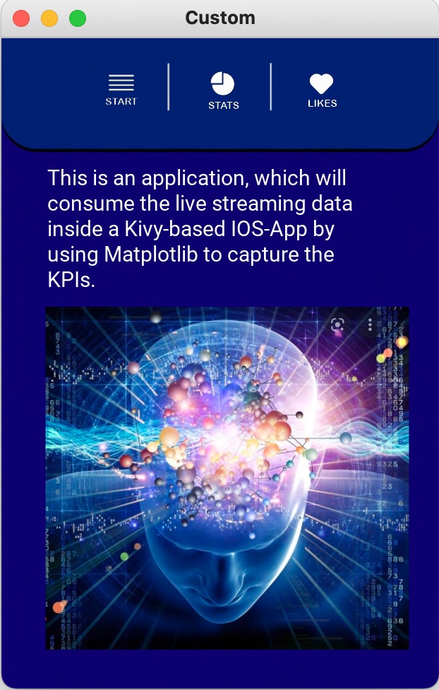
| text: "This is an application, which will consume the live streaming data inside a Kivy-based IOS-App by using Matplotlib to capture the KPIs." | |
| text_size: self.width + 350, None | |
| height: self.texture_size[1] | |
| halign: "left" | |
| valign: "bottom" | |
| pos_hint: {'center_x':2.9,'center_y':6.5} | |
| Image: | |
| id: homesc | |
| pos_hint: {'right':6, 'top':5.4} | |
| size_hint: None, None | |
| size: 560, 485 | |
| source: "Background/FP.jpeg" | |
| Screen: | |
| name: "background_2" | |
| Image: | |
| source: "Background/Background_2.png" | |
| allow_stretch: True | |
| keep_ratio: True | |
| size_hint_y: None | |
| size_hint_x: None | |
| width: self.parent.width | |
| height: self.parent.width/self.image_ratio | |
| FloatLayout: | |
| Label: | |
| text: "Please find the realtime IoT-device Live Statistics:" | |
| text_size: self.width + 430, None | |
| height: self.texture_size[1] | |
| halign: "left" | |
| valign: "top" | |
| pos_hint: {'center_x':3.0,'center_y':7.0} | |
| Label: | |
| text: "DC to Servo Min Ratio:" | |
| text_size: self.width + 430, None | |
| height: self.texture_size[1] | |
| halign: "left" | |
| valign: "top" | |
| pos_hint: {'center_x':3.0,'center_y':6.2} | |
| Label: | |
| id: dynMin | |
| text: "100" | |
| text_size: self.width + 430, None | |
| height: self.texture_size[1] | |
| halign: "left" | |
| valign: "top" | |
| pos_hint: {'center_x':6.2,'center_y':6.2} | |
| Label: | |
| text: "DC Motor:" | |
| text_size: self.width + 430, None | |
| height: self.texture_size[1] | |
| halign: "left" | |
| valign: "top" | |
| pos_hint: {'center_x':6.8,'center_y':5.4} | |
| Label: | |
| text: "(MAX)" | |
| text_size: self.width + 430, None | |
| height: self.texture_size[1] | |
| halign: "left" | |
| valign: "top" | |
| pos_hint: {'center_x':6.8,'center_y':5.0} | |
| Label: | |
| id: dynDC | |
| text: "100" | |
| text_size: self.width + 430, None | |
| height: self.texture_size[1] | |
| halign: "left" | |
| valign: "top" | |
| pos_hint: {'center_x':6.8,'center_y':4.6} | |
| Label: | |
| text: " ——- Vs ——- " | |
| text_size: self.width + 430, None | |
| height: self.texture_size[1] | |
| halign: "left" | |
| valign: "top" | |
| pos_hint: {'center_x':6.8,'center_y':4.0} | |
| Label: | |
| text: "Servo Motor:" | |
| text_size: self.width + 430, None | |
| height: self.texture_size[1] | |
| halign: "left" | |
| valign: "top" | |
| pos_hint: {'center_x':6.8,'center_y':3.4} | |
| Label: | |
| text: "(MAX)" | |
| text_size: self.width + 430, None | |
| height: self.texture_size[1] | |
| halign: "left" | |
| valign: "top" | |
| pos_hint: {'center_x':6.8,'center_y':3.0} | |
| Label: | |
| id: dynServo | |
| text: "100" | |
| text_size: self.width + 430, None | |
| height: self.texture_size[1] | |
| halign: "left" | |
| valign: "top" | |
| pos_hint: {'center_x':6.8,'center_y':2.6} | |
| FloatLayout: | |
| id: box | |
| size: 400, 550 | |
| pos: 200, 300 | |
| Screen: | |
| name: "background_3" | |
| Image: | |
| source: "Background/Background_3.png" | |
| allow_stretch: True | |
| keep_ratio: True | |
| size_hint_y: None | |
| size_hint_x: None | |
| width: self.parent.width | |
| height: self.parent.width/self.image_ratio | |
| FloatLayout: | |
| orientation: 'vertical' | |
| Label: | |
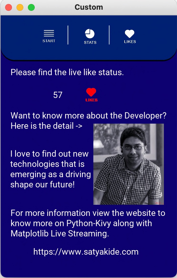
| text: "Please find the live like status." | |
| text_size: self.width + 350, None | |
| height: self.texture_size[1] | |
| halign: "left" | |
| valign: "bottom" | |
| pos_hint: {'center_x':2.6,'center_y':7.2} | |
| Label: | |
| id: dynVal | |
| text: "100" | |
| text_size: self.width + 350, None | |
| height: self.texture_size[1] | |
| halign: "left" | |
| valign: "bottom" | |
| pos_hint: {'center_x':4.1,'center_y':6.4} | |
| Image: | |
| id: lk_img_1 | |
| pos_hint: {'center_x':3.2, 'center_y':6.4} | |
| size_hint: None, None | |
| size: 460, 285 | |
| source: "Background/Likes_Btn_R.png" | |
| Label: | |
| text: "Want to know more about the Developer? Here is the detail ->" | |
| text_size: self.width + 450, None | |
| height: self.texture_size[1] | |
| halign: "left" | |
| valign: "bottom" | |
| pos_hint: {'center_x':3.1,'center_y':5.5} | |
| Label: | |
| text: "I love to find out new technologies that is emerging as a driving force & shape our future!" | |
| text_size: self.width + 290, None | |
| height: self.texture_size[1] | |
| halign: "left" | |
| valign: "bottom" | |
| pos_hint: {'center_x':2.3,'center_y':3.8} | |
| Label: | |
| text: "For more information view the website to know more on Python-Kivy along with Matplotlib Live Streaming." | |
| text_size: self.width + 450, None | |
| height: self.texture_size[1] | |
| halign: "left" | |
| valign: "bottom" | |
| pos_hint: {'center_x':3.1,'center_y':1.9} | |
| Image: | |
| id: avatar | |
| pos_hint: {'right':6.8, 'top':5.4} | |
| size_hint: None, None | |
| size: 460, 285 | |
| source: "Background/Me.jpeg" | |
| Label: | |
| text: "https://www.satyakide.com" | |
| text_size: self.width + 350, None | |
| height: self.texture_size[1] | |
| halign: "left" | |
| valign: "bottom" | |
| pos_hint: {'center_x':3.4,'center_y':0.9} | |
| Image: | |
| source: "Background/Top_Bar.png" | |
| size: 620, 175 | |
| pos: 0, root.height – 535 | |
| Button: | |
| #: set val 'Start' | |
| size: 112.5, 75 | |
| pos: root.width/2-190, root.height-120 | |
| background_color: 1,1,1,0 | |
| on_press: root.pressed(self, val, sm) | |
| on_release: root.released(self, val) | |
| Image: | |
| id: s_img | |
| text: val | |
| source: "Background/Start_Btn.png" | |
| center_x: self.parent.center_x – 260 | |
| center_y: self.parent.center_y – 415 | |
| Button: | |
| #: set val2 'Stats' | |
| size: 112.5, 75 | |
| pos: root.width/2-55, root.height-120 | |
| background_color: 1,1,1,0 | |
| on_press: root.pressed(self, val2, sm) | |
| on_release: root.released(self, val2) | |
| Image: | |
| id: st_img | |
| text: val2 | |
| source: "Background/Stats_Btn.png" | |
| center_x: self.parent.center_x – 250 | |
| center_y: self.parent.center_y – 415 | |
| Button: | |
| #: set val3 'Likes' | |
| size: 112.5, 75 | |
| pos: root.width/2+75, root.height-120 | |
| background_color: 1,1,1,0 | |
| on_press: root.pressed(self, val3, sm) | |
| on_release: root.released(self, val3) | |
| Image: | |
| id: lk_img | |
| text: val3 | |
| source: "Background/Likes_Btn.png" | |
| center_x: self.parent.center_x – 240 | |
| center_y: self.parent.center_y – 415 |
To understand this, one needs to learn how to prepare a Kivy design layout using the KV-language. You can develop the same using native-python code as well. However, I wanted to explore this language & not to mention that this is the preferred way of doing a front-end GUI design in Kivy.
Like any graphical interface, one needs to understand the layouts & the widgets that you are planning to use or build. For that, please go through the following critical documentation link on Kivy Layouts. Please go through this if you are doing this for the first time.
To pinpoint the conversation, I would like to present the documentation segment from the official site in the given picture –

Since we’ve used our custom buttons & top bars, the most convenient GUI layouts will be FloatLayout for our use case. By using that layout, we can conveniently position our widgets at any random place as per our needs. At the same time, one can use nested layouts by combining different types of arrangements under another.
Some of the key lines from the above scripting files will be –
Screen:
  name: "background_1"
  Image:
      source: "Background/Background_1.png"
      allow_stretch: True
      keep_ratio: True
      size_hint_y: None
      size_hint_x: None
      width: self.parent.width
      height: self.parent.width/self.image_ratio
      FloatLayout:
          orientation: 'vertical'
          Label:
              text: "This is an application, which will consume the live streaming data inside a Kivy-based IOS-App by using Matplotlib to capture the KPIs."
              text_size: self.width + 350, None
              height: self.texture_size[1]
              halign: "left"
              valign: "bottom"
              pos_hint: {'center_x':2.9,'center_y':6.5}
          Image:
              id: homesc
              pos_hint: {'right':6, 'top':5.4}
              size_hint: None, None
              size: 560, 485
              source: "Background/FP.jpeg"
Let us understand what we discussed here & try to map that with the image.

From the above image now, you can understand how we placed the label & image into our custom positions to create a lean & clean interface.
Image:
      source: "Background/Top_Bar.png"
      size: 620, 175
      pos: 0, root.height - 535

  Button:
      #: set val 'Start'
      size: 112.5, 75
      pos: root.width/2-190, root.height-120
      background_color: 1,1,1,0
      on_press: root.pressed(self, val, sm)
      on_release: root.released(self, val)
      Image:
          id: s_img
          text: val
          source: "Background/Start_Btn.png"
          center_x: self.parent.center_x - 260
          center_y: self.parent.center_y - 415

  Button:
      #: set val2 'Stats'
      size: 112.5, 75
      pos: root.width/2-55, root.height-120
      background_color: 1,1,1,0
      on_press: root.pressed(self, val2, sm)
      on_release: root.released(self, val2)
      Image:
          id: st_img
          text: val2
          source: "Background/Stats_Btn.png"
          center_x: self.parent.center_x - 250
          center_y: self.parent.center_y - 415

  Button:
      #: set val3 'Likes'
      size: 112.5, 75
      pos: root.width/2+75, root.height-120
      background_color: 1,1,1,0
      on_press: root.pressed(self, val3, sm)
      on_release: root.released(self, val3)
      Image:
          id: lk_img
          text: val3
          source: "Background/Likes_Btn.png"
          center_x: self.parent.center_x - 240
          center_y: self.parent.center_y - 415
Let us understand the custom buttons mapped in our Apps.

So, these are custom buttons. We placed them into specific positions & sizes by mentioning the appropriate size & position coordinates & then assigned the button methods (on_press & on_release).
However, these button methods will be present inside the main python script, which we’ll discuss after this segment.
3. main.py (Consuming Streaming data from Ably channels & captured IoT events from the simulator & publish them in Kivy-based iOS App through measured KPIs.)
This file contains hidden or bidirectional Unicode text that may be interpreted or compiled differently than what appears below. To review, open the file in an editor that reveals hidden Unicode characters.
Learn more about bidirectional Unicode characters
| ############################################## | |
| #### Updated By: SATYAKI DE #### | |
| #### Updated On: 12-Nov-2021 #### | |
| #### #### | |
| #### Objective: Consuming Streaming data #### | |
| #### from Ably channels & captured IoT #### | |
| #### events from the simulator & publish #### | |
| #### them in Kivy-I/OS App through #### | |
| #### measured KPIs. #### | |
| #### #### | |
| ############################################## | |
| from kivy.app import App | |
| from kivy.uix.widget import Widget | |
| from kivy.lang import Builder | |
| from kivy.uix.boxlayout import BoxLayout | |
| from kivy.uix.floatlayout import FloatLayout | |
| from kivy.clock import Clock | |
| from kivy.core.window import Window | |
| from kivymd.app import MDApp | |
| import datetime as dt | |
| import datetime | |
| from kivy.properties import StringProperty | |
| from kivy.vector import Vector | |
| import regex as re | |
| import os | |
| os.environ["KIVY_IMAGE"]="pil" | |
| import platform as pl | |
| import matplotlib.pyplot as plt | |
| import pandas as p | |
| from matplotlib.patches import Rectangle | |
| from matplotlib import use as mpl_use | |
| mpl_use('module://kivy.garden.matplotlib.backend_kivy') | |
| plt.style.use('fivethirtyeight') | |
| # Consuming data from Ably Queue | |
| from ably import AblyRest | |
| # Main Class to consume streaming | |
| import clsStreamConsume as ca | |
| # Create the instance of the Covid API Class | |
| x1 = ca.clsStreamConsume() | |
| var1 = datetime.datetime.now().strftime("%Y-%m-%d_%H-%M-%S") | |
| print('*' *60) | |
| DInd = 'Y' | |
| Window.size = (310, 460) | |
| Curr_Path = os.path.dirname(os.path.realpath(__file__)) | |
| os_det = pl.system() | |
| if os_det == "Windows": | |
| sep = '\\' | |
| else: | |
| sep = '/' | |
| def getRealTimeIoT(): | |
| try: | |
| # Let's pass this to our map section | |
| df = x1.conStream(var1, DInd) | |
| print('Data:') | |
| print(str(df)) | |
| return df | |
| except Exception as e: | |
| x = str(e) | |
| print(x) | |
| df = p.DataFrame() | |
| return df | |
| class MainInterface(FloatLayout): | |
| def __init__(self, **kwargs): | |
| super().__init__(**kwargs) | |
| self.data = getRealTimeIoT() | |
| self.likes = 0 | |
| self.dcMotor = 0 | |
| self.servoMotor = 0 | |
| self.minRatio = 0 | |
| plt.subplots_adjust(bottom=0.19) | |
| #self.fig, self.ax = plt.subplots(1,1, figsize=(6.5,10)) | |
| self.fig, self.ax = plt.subplots() | |
| self.mpl_canvas = self.fig.canvas | |
| def on_data(self, *args): | |
| self.ax.clear() | |
| self.data = getRealTimeIoT() | |
| self.ids.lk_img_1.source = Curr_Path + sep + 'Background' + sep + "Likes_Btn.png" | |
| self.likes = self.getMaxLike(self.data) | |
| self.ids.dynVal.text = str(self.likes) | |
| self.ids.lk_img_1.source = '' | |
| self.ids.lk_img_1.source = Curr_Path + sep + 'Background' + sep + "Likes_Btn_R.png" | |
| self.dcMotor = self.getMaxDCMotor(self.data) | |
| self.ids.dynDC.text = str(self.dcMotor) | |
| self.servoMotor = self.getMaxServoMotor(self.data) | |
| self.ids.dynServo.text = str(self.servoMotor) | |
| self.minRatio = self.getDc2ServoMinRatio(self.data) | |
| self.ids.dynMin.text = str(self.minRatio) | |
| x = self.data['x_value'] | |
| y1 = self.data['total_1'] | |
| y2 = self.data['total_2'] | |
| self.ax.plot(x, y1, label='Channel 1', linewidth=5.0) | |
| self.ax.plot(x, y2, label='Channel 2', linewidth=5.0) | |
| self.mpl_canvas.draw_idle() | |
| box = self.ids.box | |
| box.clear_widgets() | |
| box.add_widget(self.mpl_canvas) | |
| return self.data | |
| def getMaxLike(self, df): | |
| payload = df['x_value'] | |
| a1 = str(payload.agg(['max'])) | |
| max_val = int(re.search(r'\d+', a1)[0]) | |
| return max_val | |
| def getMaxDCMotor(self, df): | |
| payload = df['total_1'] | |
| a1 = str(payload.agg(['max'])) | |
| max_val = int(re.search(r'\d+', a1)[0]) | |
| return max_val | |
| def getMaxServoMotor(self, df): | |
| payload = df['total_2'] | |
| a1 = str(payload.agg(['max'])) | |
| max_val = int(re.search(r'\d+', a1)[0]) | |
| return max_val | |
| def getMinDCMotor(self, df): | |
| payload = df['total_1'] | |
| a1 = str(payload.agg(['min'])) | |
| min_val = int(re.search(r'\d+', a1)[0]) | |
| return min_val | |
| def getMinServoMotor(self, df): | |
| payload = df['total_2'] | |
| a1 = str(payload.agg(['min'])) | |
| min_val = int(re.search(r'\d+', a1)[0]) | |
| return min_val | |
| def getDc2ServoMinRatio(self, df): | |
| minDC = self.getMinDCMotor(df) | |
| minServo = self.getMinServoMotor(df) | |
| min_ratio = round(float(minDC/minServo), 5) | |
| return min_ratio | |
| def update(self, *args): | |
| self.data = self.on_data(self.data) | |
| def pressed(self, instance, inText, SM): | |
| if str(inText).upper() == 'START': | |
| instance.parent.ids.s_img.source = Curr_Path + sep + 'Background' + sep + "Pressed_Start_Btn.png" | |
| print('In Pressed: ', str(instance.parent.ids.s_img.text).upper()) | |
| if ((SM.current == "background_2") or (SM.current == "background_3")): | |
| SM.transition.direction = "right" | |
| SM.current= "background_1" | |
| Clock.unschedule(self.update) | |
| self.remove_widget(self.mpl_canvas) | |
| elif str(inText).upper() == 'STATS': | |
| instance.parent.ids.st_img.source = Curr_Path + sep + 'Background' + sep + "Pressed_Stats_Btn.png" | |
| print('In Pressed: ', str(instance.parent.ids.st_img.text).upper()) | |
| if (SM.current == "background_1"): | |
| SM.transition.direction = "left" | |
| elif (SM.current == "background_3"): | |
| SM.transition.direction = "right" | |
| SM.current= "background_2" | |
| Clock.schedule_interval(self.update, 0.1) | |
| else: | |
| instance.parent.ids.lk_img.source = Curr_Path + sep + 'Background' + sep + "Pressed_Likes_Btn.png" | |
| print('In Pressed: ', str(instance.parent.ids.lk_img.text).upper()) | |
| if ((SM.current == "background_1") or (SM.current == "background_2")): | |
| SM.transition.direction = "left" | |
| SM.current= "background_3" | |
| Clock.schedule_interval(self.update, 0.1) | |
| instance.parent.ids.dynVal.text = str(self.likes) | |
| instance.parent.ids.dynDC.text = str(self.dcMotor) | |
| instance.parent.ids.dynServo.text = str(self.servoMotor) | |
| instance.parent.ids.dynMin.text = str(self.minRatio) | |
| self.remove_widget(self.mpl_canvas) | |
| def released(self, instance, inrText): | |
| if str(inrText).upper() == 'START': | |
| instance.parent.ids.s_img.source = Curr_Path + sep + 'Background' + sep + "Start_Btn.png" | |
| print('Released: ', str(instance.parent.ids.s_img.text).upper()) | |
| elif str(inrText).upper() == 'STATS': | |
| instance.parent.ids.st_img.source = Curr_Path + sep + 'Background' + sep + "Stats_Btn.png" | |
| print('Released: ', str(instance.parent.ids.st_img.text).upper()) | |
| else: | |
| instance.parent.ids.lk_img.source = Curr_Path + sep + 'Background' + sep + "Likes_Btn.png" | |
| print('Released: ', str(instance.parent.ids.lk_img.text).upper()) | |
| class CustomApp(MDApp): | |
| def build(self): | |
| return MainInterface() | |
| if __name__ == "__main__": | |
| custApp = CustomApp() | |
| custApp.run() |
Let us explore the main script now.
def getRealTimeIoT():
    try:
        # Let's pass this to our map section
        df = x1.conStream(var1, DInd)

        print('Data:')
        print(str(df))

        return df
    except Exception as e:
        x = str(e)
        print(x)

        df = p.DataFrame()

        return df
The above function will invoke the streaming class to consume the mock IoT live events as a pandas dataframe from the Ably queue.
class MainInterface(FloatLayout):

    def __init__(self, **kwargs):
        super().__init__(**kwargs)
        self.data = getRealTimeIoT()
        self.likes = 0
        self.dcMotor = 0
        self.servoMotor = 0
        self.minRatio = 0
        plt.subplots_adjust(bottom=0.19)

        #self.fig, self.ax = plt.subplots(1,1, figsize=(6.5,10))
        self.fig, self.ax = plt.subplots()
        self.mpl_canvas = self.fig.canvas
Application is instantiating the main class & assignments of all the critical variables, including the matplotlib class.
    def pressed(self, instance, inText, SM):

        if str(inText).upper() == 'START':
            instance.parent.ids.s_img.source = Curr_Path + sep + 'Background' + sep + "Pressed_Start_Btn.png"
            print('In Pressed: ', str(instance.parent.ids.s_img.text).upper())
            if ((SM.current == "background_2") or (SM.current == "background_3")):
                SM.transition.direction = "right"
            SM.current= "background_1"
            Clock.unschedule(self.update)
            self.remove_widget(self.mpl_canvas)
We’ve taken one of the button events & captured how the application will behave once someone clicks the Start button & how it will bring all the corresponding elements of a static page. It also explained the transition type between screens.
        elif str(inText).upper() == 'STATS':

            instance.parent.ids.st_img.source = Curr_Path + sep + 'Background' + sep + "Pressed_Stats_Btn.png"
            print('In Pressed: ', str(instance.parent.ids.st_img.text).upper())
            if (SM.current == "background_1"):
                SM.transition.direction = "left"
            elif (SM.current == "background_3"):
                SM.transition.direction = "right"
            SM.current= "background_2"
            Clock.schedule_interval(self.update, 0.1)
The next screen invokes the dynamic & real-time content. So, please pay extra attention to the following line –
Clock.schedule_interval(self.update, 0.1)
This line will invoke the update function, which looks like –
    def update(self, *args):
        self.data = self.on_data(self.data)
Here is the logic for the update function, which will invoke another function named – “on_data“.
    def on_data(self, *args):
        self.ax.clear()
        self.data = getRealTimeIoT()

        self.ids.lk_img_1.source = Curr_Path + sep + 'Background' + sep + "Likes_Btn.png"
        self.likes = self.getMaxLike(self.data)
        self.ids.dynVal.text = str(self.likes)
        self.ids.lk_img_1.source = ''
        self.ids.lk_img_1.source = Curr_Path + sep + 'Background' + sep + "Likes_Btn_R.png"

        self.dcMotor = self.getMaxDCMotor(self.data)
        self.ids.dynDC.text = str(self.dcMotor)

        self.servoMotor = self.getMaxServoMotor(self.data)
        self.ids.dynServo.text = str(self.servoMotor)

        self.minRatio = self.getDc2ServoMinRatio(self.data)
        self.ids.dynMin.text = str(self.minRatio)

        x = self.data['x_value']
        y1 = self.data['total_1']
        y2 = self.data['total_2']

        self.ax.plot(x, y1, label='Channel 1', linewidth=5.0)
        self.ax.plot(x, y2, label='Channel 2', linewidth=5.0)

        self.mpl_canvas.draw_idle()

        box = self.ids.box
        box.clear_widgets()
        box.add_widget(self.mpl_canvas)

        return self.data
The above crucial line shows how we capture the live calculation & assign them into matplotlib plots & finally assign that figure canvas of matplotlib to a box widget as per our size & display the change content whenever it invokes this method.
Rests of the functions are pretty self-explanatory. So, I’m not going to discuss them.
Run:
Let’s run the app & see the output –
STEP – 1

STEP – 2

STEP – 3

So, we’ve done it.
You will get the complete codebase in the following Github link.
I’ll bring some more exciting topic in the coming days from the Python verse. Please share & subscribe my post & let me know your feedback.
Till then, Happy Avenging!
Note: All the data & scenario posted here are representational data & scenarios & available over the internet & for educational purpose only. Some of the images (except my photo) that we’ve used are available over the net. We don’t claim the ownership of these images. There is an always room for improvement & especially all the GUI components size & position that will be dynamic in nature by defining self.width along with some constant values.


You must be logged in to post a comment.