
As we’ve started explaining, the importance & usage of Stable Defussion in our previous post:
Enabling & Exploring Stable Defussion – Part 1
In today’s post, we’ll discuss another approach, where we built the custom Python-based SDK solution that consumes HuggingFace Library, which generates video out of the supplied prompt.
But, before that, let us view the demo generated from a custom solution.
Isn’t it exciting? Let us dive deep into the details.
FLOW:
Let us understand basic flow of events for the custom solution –

So, the application will interact with the python-sdk like “stable-diffusion-3.5-large” & “dreamshaper-xl-1-0”, which is available in HuggingFace. As part of the process, these libraries will load all the large models inside the local laptop that require some time depend upon the bandwidth of your internet.
Before we even deep dive into the code, let us understand the flow of Python scripts as shown below:

From the above diagram, we can understand that the main application will be triggered by “generateText2Video.py”. As you can see that “clsConfigClient.py” has all the necessary parameter information that will be supplied to all the scripts.
“generateText2Video.py” will trigger the main class named “clsText2Video.py”, which then calls all the subsequent classes.
Great! Since we now have better visibility of the script flow, let’s examine the key snippets individually.
CODE:
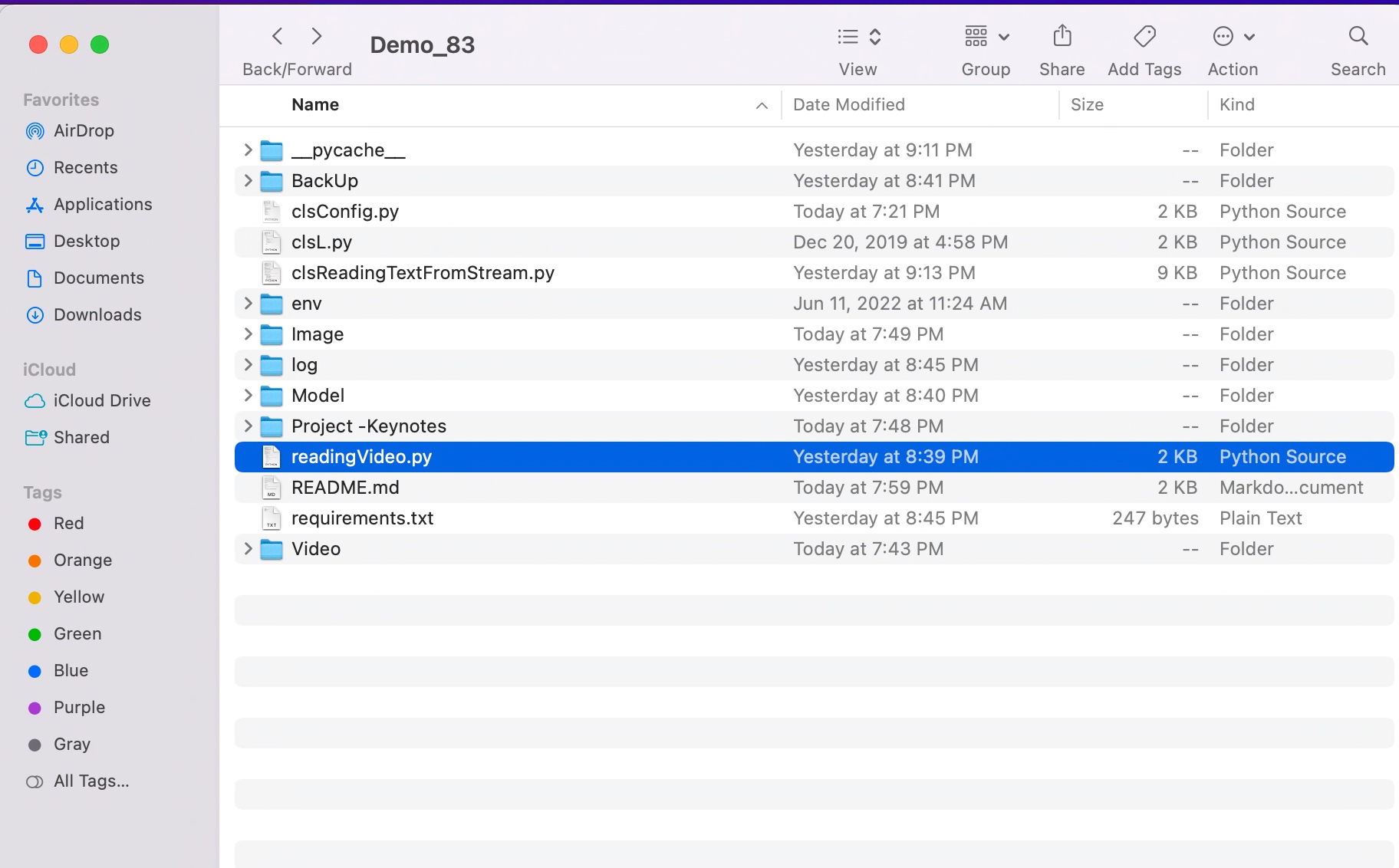
clsText2Video.py (The main class that initiates the fellow classes to convert from prompt to video):
class clsText2Video:
    def __init__(self, model_id_1, model_id_2, output_path, filename, vidfilename, fps, force_cpu=False):
        self.model_id_1 = model_id_1
        self.model_id_2 = model_id_2
        self.output_path = output_path
        self.filename = filename
        self.vidfilename = vidfilename
        self.force_cpu = force_cpu
        self.fps = fps

        # Initialize in main process
        os.environ["TOKENIZERS_PARALLELISM"] = "true"
        self.r1 = cm.clsMaster(force_cpu)
        self.torch_type = self.r1.getTorchType()

        torch.mps.empty_cache()
        self.pipe = self.r1.getText2ImagePipe(self.model_id_1, self.torch_type)
        self.pipeline = self.r1.getImage2VideoPipe(self.model_id_2, self.torch_type)

        self.text2img = cti.clsText2Image(self.pipe, self.output_path, self.filename)
        self.img2vid = civ.clsImage2Video(self.pipeline)

    def getPrompt2Video(self, prompt):
        try:
            input_image = self.output_path + self.filename
            target_video = self.output_path + self.vidfilename

            if self.text2img.genImage(prompt) == 0:
                print('Pass 1: Text to intermediate images generated!')

                if self.img2vid.genVideo(prompt, input_image, target_video, self.fps) == 0:
                    print('Pass 2: Successfully generated!')
                    return 0
            return 1
        except Exception as e:
            print(f"\nAn unexpected error occurred: {str(e)}")
            return 1
Now, let us interpret:
1. CLASS INSTANTIATION:
This is the initialization method for the class. It does the following:
- Sets up configurations like model IDs, output paths, filenames, video filename, frames per second (fps), and whether to use the CPU (
force_cpu). - Configures an environment variable for tokenizer parallelism.
- Initializes helper classes (
clsMaster) to manage system resources and retrieve appropriate PyTorch settings. - Creates two pipelines:
pipe: For converting text to images using the first model.pipeline: For converting images to video using the second model.
- Initializes
text2imgandimg2vidobjects:text2imghandles text-to-image conversions.img2vidhandles image-to-video conversions.
2. getPrompt2Video(prompt)
This method generates a video from a text prompt in two steps:
- Text-to-Image Conversion:
- Calls
genImage(prompt)using thetext2imgobject to create an intermediate image file. - If successful, it prints confirmation.
- Calls
- Image-to-Video Conversion:
- Uses the
img2vidobject to convert the intermediate image into a video file. - Includes the input image path, target video path, and frames per second (fps).
- If successful, it prints confirmation.
- Uses the
- If either step fails, the method returns
1. - Logs any unexpected errors and returns
1in such cases.
clsMaster.py (This class packaged all the necessary common capabilities that can be used from a single class)
# Set device for Apple Silicon GPU
def setup_gpu(force_cpu=False):
    if not force_cpu and torch.backends.mps.is_available() and torch.backends.mps.is_built():
        print('Running on Apple Silicon MPS GPU!')
        return torch.device("mps")
    return torch.device("cpu")

######################################
####         Global Flag      ########
######################################

class clsMaster:
    def __init__(self, force_cpu=False):
        self.device = setup_gpu(force_cpu)

    def getTorchType(self):
        try:
            # Check if MPS (Apple Silicon GPU) is available
            if not torch.backends.mps.is_available():
                torch_dtype = torch.float32
                raise RuntimeError("MPS (Metal Performance Shaders) is not available on this system.")
            else:
                torch_dtype = torch.float16

            return torch_dtype
        except Exception as e:
            torch_dtype = torch.float16
            print(f'Error: {str(e)}')

            return torch_dtype

    def getText2ImagePipe(self, model_id, torchType):
        try:
            device = self.device

            torch.mps.empty_cache()
            self.pipe = StableDiffusion3Pipeline.from_pretrained(model_id, torch_dtype=torchType, use_safetensors=True, variant="fp16",).to(device)

            return self.pipe
        except Exception as e:
            x = str(e)
            print('Error: ', x)

            torch.mps.empty_cache()
            self.pipe = StableDiffusion3Pipeline.from_pretrained(model_id, torch_dtype=torchType,).to(device)

            return self.pipe

    def getImage2VideoPipe(self, model_id, torchType):
        try:
            device = self.device

            torch.mps.empty_cache()
            self.pipeline = StableDiffusionXLImg2ImgPipeline.from_pretrained(model_id, torch_dtype=torchType, use_safetensors=True, use_fast=True).to(device)

            return self.pipeline
        except Exception as e:
            x = str(e)
            print('Error: ', x)

            torch.mps.empty_cache()
            self.pipeline = StableDiffusionXLImg2ImgPipeline.from_pretrained(model_id, torch_dtype=torchType).to(device)

            return self.pipeline
Let us interpret:
1. setup_gpu(force_cpu=False)
This function determines whether to use the Apple Silicon GPU (MPS) or the CPU:
- If
force_cpuisFalseand the MPS GPU is available, it sets the device to “mps” (Apple GPU) and prints a message. - Otherwise, it defaults to the CPU.
2. CLASS INSTANTIATION (force_cpu=False)
This is the initializer for the clsMaster class:
- It sets the
deviceto either GPU or CPU using thesetup_gpufunction (mentioned above) based on theforce_cpuflag.
3. getTorchType
This method determines the PyTorch data type to use:
- Checks if MPS GPU is available:
- If available, uses
torch.float16for optimized performance. - If unavailable, defaults to
torch.float32and raises a warning.
- If available, uses
- Handles errors gracefully by defaulting to
torch.float16and printing the error.
4. getText2ImagePipe(model_id, torchType)
This method initializes a text-to-image pipeline:
- Loads the Stable Diffusion model with the given
model_idandtorchType. - Configures it for MPS GPU or CPU, based on the device.
- Clears the GPU cache before loading the model to optimize memory usage.
- If an error occurs, attempts to reload the pipeline without safetensors.
5. getImage2VideoPipe(model_id, torchType)
This method initializes an image-to-video pipeline:
- Similar to
getText2ImagePipe, it loads the Stable Diffusion XL Img2Img pipeline with the specifiedmodel_idandtorchType. - Configures it for MPS GPU or CPU and clears the cache before loading.
- On error, reloads the pipeline without additional optimization settings and prints the error.
Let us continue this in the next post:
Enabling & Exploring Stable Defussion – Part 3
Till then, Happy Avenging! 🙂
Note: All the data & scenarios posted here are representational data & scenarios & available over the internet & for educational purposes only. There is always room for improvement in this kind of model & the solution associated with it. I’ve shown the basic ways to achieve the same for educational purposes only.


You must be logged in to post a comment.