Tag: machine-learning

This week we’re planning to touch on one of the exciting posts of visually reading characters from WebCAM & predict the letters using CNN methods. Before we dig deep, why don’t we see the demo run first?

Isn’t it fascinating? As we can see, the computer can record events and read like humans. And, thanks to the brilliant packages available in Python, which can help us predict the correct letter out of an Image.

What do we need to test it out?

1. Preferably an external WebCAM.
2. A moderate or good Laptop to test out this.
3. Python 
4. And a few other packages that we’ll mention next block.

What Python packages do we need?

Some of the critical packages that we must need to test out this application are –

cmake==3.22.1
dlib==19.19.0
face-recognition==1.3.0
face-recognition-models==0.3.0
imutils==0.5.3
jsonschema==4.4.0
keras==2.7.0
Keras-Preprocessing==1.1.2
matplotlib==3.5.1
matplotlib-inline==0.1.3
oauthlib==3.1.1
opencv-contrib-python==4.1.2.30
opencv-contrib-python-headless==4.4.0.46
opencv-python==4.5.5.62
opencv-python-headless==4.5.5.62
pickleshare==0.7.5
Pillow==9.0.0
python-dateutil==2.8.2
requests==2.27.1
requests-oauthlib==1.3.0
scikit-image==0.19.1
scikit-learn==1.0.2
tensorboard==2.7.0
tensorboard-data-server==0.6.1
tensorboard-plugin-wit==1.8.1
tensorflow==2.7.0
tensorflow-estimator==2.7.0
tensorflow-io-gcs-filesystem==0.23.1
tqdm==4.62.3

What is CNN?

In deep learning, a convolutional neural network (CNN/ConvNet) is a class of deep neural networks most commonly applied to analyze visual imagery.

We can understand from the above picture that a CNN generally takes an image as input. The neural network analyzes each pixel separately. The weights and biases of the model are then tweaked to detect the desired letters (In our use case) from the image. Like other algorithms, the data also has to pass through pre-processing stage. However, a CNN needs relatively less pre-processing than most other Deep Learning algorithms.

If you want to know more about this, there is an excellent article on CNN with some on-point animations explaining this concept. Please read it here.

Where do we get the data sets for our testing?

For testing, we are fortunate enough to have Kaggle with us. We have received a wide variety of sample data, which you can get from here.

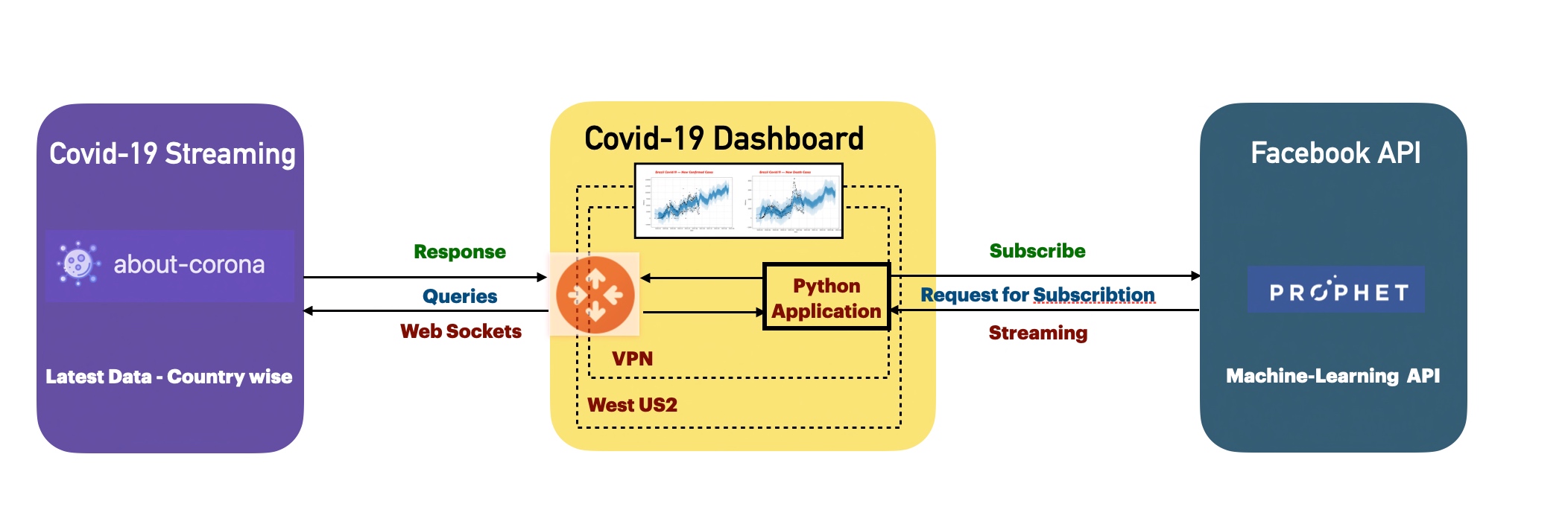
Our use-case:

From the above diagram, one can see that the python application will consume a live video feed of any random letters (both printed & handwritten) & predict the character as part of the machine learning model that we trained.

Code:

1. clsConfig.py (Configuration file for the entire application.)

Important parameters that we need to follow from the above snippets are –

'testRatio':0.2,
'valRatio':0.2,
'epochsVal':8,
'activationType':'relu',
'activationType2':'softmax',
'numOfClasses':26,
'kernelSize':(3, 3),
'poolSize':(2, 2),
'word_dict':{0:'A',1:'B',2:'C',3:'D',4:'E',5:'F',6:'G',7:'H',8:'I',9:'J',10:'K',11:'L',12:'M',13:'N',14:'O',15:'P',16:'Q',17:'R',18:'S',19:'T',20:'U',21:'V',22:'W',23:'X', 24:'Y',25:'Z'},

Since we have 26 letters, we have classified it as 26 in the numOfClasses.

Since we are talking about characters, we had to come up with a process of identifying each character as numbers & then processing our entire logic. Hence, the above parameter named word_dict captured all the characters in a python dictionary & stored them. Moreover, the application translates the final number output to more appropriate characters as the prediction.

2. clsAlphabetReading.py (Main training class to teach the model to predict alphabets from visual reader.)

Some of the key snippets from the above scripts are –

x = df_HW_Alphabet.drop('0',axis = 1)
y = df_HW_Alphabet['0']

In the above snippet, we have split the data into images & their corresponding labels.

X_Train, X_Test, Y_Train, Y_Test = train_test_split(x, y, test_size = testRatio)
X_Train, X_Validation, Y_Train, Y_Validation = train_test_split(X_Train, Y_Train, test_size = valRatio)

X_Train = np.reshape(X_Train.values, (X_Train.shape[0], reshapeVal, reshapeVal))
X_Test = np.reshape(X_Test.values, (X_Test.shape[0], reshapeVal, reshapeVal))
X_Validation = np.reshape(X_Validation.values, (X_Validation.shape[0], reshapeVal, reshapeVal))


print("Train Data Shape: ", X_Train.shape)
print("Test Data Shape: ", X_Test.shape)
print("Validation Data shape: ", X_Validation.shape)

We are splitting the data into Train, Test & Validation sets to get more accurate predictions and reshaping the raw data into the image by consuming the 784 data columns to 28×28 pixel images.

Since we are talking about characters, we had to come up with a process of identifying The following snippet will plot the character equivalent number into a matplotlib chart & showcase the overall distribution trend after splitting.

Y_Train_Num = np.int0(y)
count = np.zeros(numOfClasses, dtype='int')
for i in Y_Train_Num:
    count[i] +=1

alphabets = []
for i in word_dict.values():
    alphabets.append(i)

fig, ax = plt.subplots(1,1, figsize=(7,7))
ax.barh(alphabets, count)

plt.xlabel("Number of elements ")
plt.ylabel("Alphabets")
plt.grid()
plt.show(block=False)
plt.pause(sleepTime)
plt.close()

Note that we have tweaked the plt.show property with (block=False). This property will enable us to continue execution without human interventions after the initial pause.

# Model reshaping the training & test dataset
X_Train = X_Train.reshape(X_Train.shape[0],X_Train.shape[1],X_Train.shape[2],1)
print("Shape of Train Data: ", X_Train.shape)

X_Test = X_Test.reshape(X_Test.shape[0], X_Test.shape[1], X_Test.shape[2],1)
print("Shape of Test Data: ", X_Test.shape)

X_Validation = X_Validation.reshape(X_Validation.shape[0], X_Validation.shape[1], X_Validation.shape[2],1)
print("Shape of Validation data: ", X_Validation.shape)

# Converting the labels to categorical values
Y_Train_Catg = to_categorical(Y_Train, num_classes = numOfClasses, dtype='int')
print("Shape of Train Labels: ", Y_Train_Catg.shape)

Y_Test_Catg = to_categorical(Y_Test, num_classes = numOfClasses, dtype='int')
print("Shape of Test Labels: ", Y_Test_Catg.shape)

Y_Validation_Catg = to_categorical(Y_Validation, num_classes = numOfClasses, dtype='int')
print("Shape of validation labels: ", Y_Validation_Catg.shape)

In the above diagram, the application did reshape all three categories of data before calling the primary CNN function.

model = Sequential()

model.add(Conv2D(filters=filterVal1, kernel_size=kernelSize, activation=activationType, input_shape=(28,28,1)))
model.add(MaxPool2D(pool_size=poolSize, strides=stridesVal))

model.add(Conv2D(filters=filterVal2, kernel_size=kernelSize, activation=activationType, padding = paddingVal1))
model.add(MaxPool2D(pool_size=poolSize, strides=stridesVal))

model.add(Conv2D(filters=filterVal3, kernel_size=kernelSize, activation=activationType, padding = paddingVal2))
model.add(MaxPool2D(pool_size=poolSize, strides=stridesVal))

model.add(Flatten())

model.add(Dense(DenkseVal2,activation = activationType))
model.add(Dense(DenkseVal3,activation = activationType))

model.add(Dense(DenkseVal1,activation = activationType2))

model.compile(optimizer = Adam(learning_rate=learningRateVal), loss='categorical_crossentropy', metrics=['accuracy'])
reduce_lr = ReduceLROnPlateau(monitor=monitorVal, factor=factorVal, patience=patienceVal1, min_lr=minLrVal)
early_stop = EarlyStopping(monitor=monitorVal, min_delta=minDeltaVal, patience=patienceVal2, verbose=verboseFlag, mode=modeInd)


fittedModel = model.fit(X_Train, Y_Train_Catg, epochs=epochsVal, callbacks=[reduce_lr, early_stop],  validation_data = (X_Validation,Y_Validation_Catg))

return (model, fittedModel)

In the above snippet, the convolution layers are followed by maxpool layers, which reduce the number of features extracted. The output of the maxpool layers and convolution layers are flattened into a vector of a single dimension and supplied as an input to the Dense layer—the CNN model prepared for training the model using the training dataset.

We have used optimization parameters like Adam, RMSProp & the application we trained for eight epochs for better accuracy & predictions.

# Displaying the accuracies & losses for train & validation set
print("Validation Accuracy :", history.history['val_accuracy'])
print("Training Accuracy :", history.history['accuracy'])
print("Validation Loss :", history.history['val_loss'])
print("Training Loss :", history.history['loss'])

# Displaying the Loss Graph
plt.figure(1)
plt.plot(history.history['loss'])
plt.plot(history.history['val_loss'])
plt.legend(['training','validation'])
plt.title('Loss')
plt.xlabel('epoch')
plt.show(block=False)
plt.pause(sleepTime1)
plt.close()

# Dsiplaying the Accuracy Graph
plt.figure(2)
plt.plot(history.history['accuracy'])
plt.plot(history.history['val_accuracy'])
plt.legend(['training','validation'])
plt.title('Accuracy')
plt.xlabel('epoch')
plt.show(block=False)
plt.pause(sleepTime1)
plt.close()

Also, we have captured the validation Accuracy & Loss & plot them into two separate graphs for better understanding.

try:
    score = model.evaluate(X_Test, Y_Test_Catg, verbose=0)
    print('Test Score = ', score[0])
    print('Test Accuracy = ', score[1])
except Exception as e:
    x = str(e)
    print('Error: ', x)

Also, the application is trying to get the accuracy of the model that we trained & validated with the training & validation data. This time we have used test data to predict the confidence score.

# Displaying some of the test images & their predicted labels
fig, ax = plt.subplots(3,3, figsize=(8,9))
axes = ax.flatten()

for i in range(9):
    axes[i].imshow(np.reshape(X_Test[i], reshapeVal1), cmap="Greys")
    pred = word_dict[np.argmax(Y_Test_Catg[i])]
    print('Prediction: ', pred)
    axes[i].set_title("Test Prediction: " + pred)
    axes[i].grid()
plt.show(block=False)
plt.pause(sleepTime1)
plt.close()

Finally, the application testing with some random test data & tried to plot the output & prediction assessment.

fileName = Curr_Path + sep + 'Model' + sep + 'model_trained_' + str(epochsVal) + '.p'
print('Model Name: ', str(fileName))

pickle_out = open(fileName, 'wb')
pickle.dump(model, pickle_out)
pickle_out.close()

As a part of the last step, the application will generate the models using a pickle package & save them under a specific location, which the reader application will use.

3. trainingVisualDataRead.py (Main application that will invoke the training class to predict alphabet through WebCam using Convolutional Neural Network (CNN).)

And the core snippet from the above script is –

x1 = ar.clsAlphabetReading()

Instantiate the main class.

r1 = x1.trainModel(debugInd, var)

The python application will invoke the class & capture the returned value inside the r1 variable.

4. readingVisualData.py (Reading the model to predict Alphabet using WebCAM.)

And the key snippet from the above code is –

cap = cv2.VideoCapture(0)
cap.set(3, width)
cap.set(4, height)

The application is reading the live video data from WebCAM. Also, set out the height & width for the video output.

fileName = Curr_Path + sep + 'Model' + sep + 'model_trained_' + str(epochsVal) + '.p'
print('Model Name: ', str(fileName))

pickle_in = open(fileName, 'rb')
model = pickle.load(pickle_in)

The application reads the model output generated as part of the previous script using the pickle package.

while True:
    status, img = cap.read()

    if status == False:
        break

The application will read the WebCAM & it exits if there is an end of video transmission or some kind of corrupt video frame.

img_copy = img.copy()

img = cv2.cvtColor(img, cv2.COLOR_BGR2RGB)
img = cv2.resize(img, imgDimension)

img_copy = cv2.GaussianBlur(img_copy, imgSmallDim, 0)
img_gray = cv2.cvtColor(img_copy, cv2.COLOR_BGR2GRAY)
bin, img_thresh = cv2.threshold(img_gray, 100, 255, cv2.THRESH_BINARY_INV)

img_final = cv2.resize(img_thresh, imgMidDim)
img_final = np.reshape(img_final, (reshapeParam1,reshapeParam2,reshapeParam2,reshapeParam1))


img_pred = word_dict[np.argmax(model.predict(img_final))]

We have initially cloned the original video frame & then it converted from BGR2GRAYSCALE while applying the threshold on it doe better prediction outcomes. Then the image has resized & reshaped for model input. Finally, the np.argmax function extracted the class index with the highest predicted probability. Furthermore, it is translated using the word_dict dictionary to an Alphabet & displayed on top of the Live View.

# Extracting Probability Values
Predict_X = model.predict(img_final)
probVal = round(np.amax(Predict_X) * 100)

Also, derive the confidence score of that probability & display that on top of the Live View.

if cv2.waitKey(1) & 0xFF == ord('q'):
    r1=0
    break

The above code will let the developer exit from this application by pressing the “Esc” or “q”-key from the keyboard & the program will terminate.

So, we’ve done it.

You will get the complete codebase in the following Github link.

I’ll bring some more exciting topic in the coming days from the Python verse. Please share & subscribe my post & let me know your feedback.

Till then, Happy Avenging! 😀

Note: All the data & scenario posted here are representational data & scenarios & available over the internet & for educational purpose only. Some of the images (except my photo) that we’ve used are available over the net. We don’t claim the ownership of these images. There is an always room for improvement & especially the prediction quality of Alphabet.