Tag: prediction

Hi Guys,

Today, I’ll be using another exciting installment of Computer Vision. Our focus will be on getting a sense of human emotions. Let me explain. This post will demonstrate how to read/detect human emotions by analyzing computer vision videos. We will be using part of a Bengali Movie called “Ganashatru (An enemy of the people)” entirely for educational purposes & also as a tribute to the great legendary director late Satyajit Roy. To know more about him, please click the following link.

Why don’t we see the demo first before jumping into the technical details?

Architecture:

Let us understand the architecture –

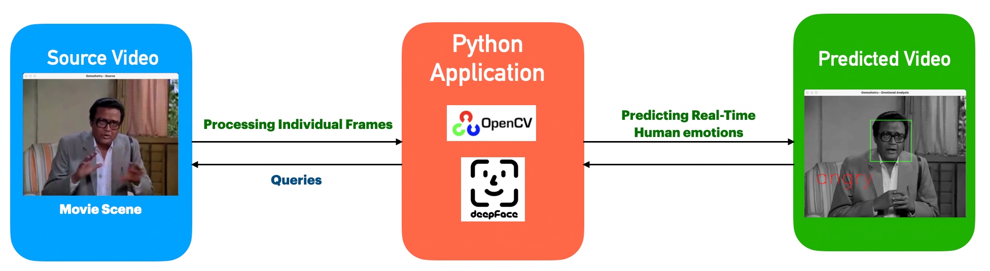
From the above diagram, one can see that the application, which uses both the Open-CV & DeepFace, analyzes individual frames from the source. Then predicts the emotions & adds the label in the target B&W frames. Finally, it creates another video by correctly mixing the source audio.

Python Packages:

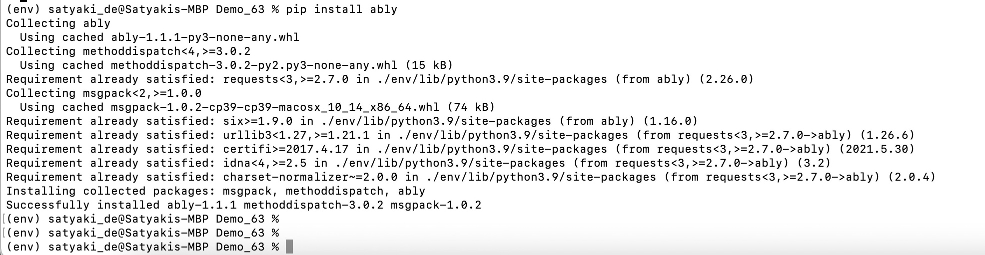
Following are the python packages that are necessary to develop this brilliant use case –

pip install deepface
pip install opencv-python
pip install ffpyplayer

CODE:

Let us now understand the code. For this use case, we will only discuss three python scripts. However, we need more than these three. However, we have already discussed them in some of the early posts. Hence, we will skip them here.

• clsConfig.py (This script will play the video along with audio in sync.)

All the above inputs are generic & used as normal parameters.

• clsFaceEmotionDetect.py (This python class will track the human emotions after splitting the audio from the video & put that label on top of the video frame.)

Key snippets from the above scripts –

def convert_video_to_audio_ffmpeg(self, video_file, output_ext="mp3"):
    try:
        """Converts video to audio directly using `ffmpeg` command
        with the help of subprocess module"""
        filename, ext = os.path.splitext(video_file)
        subprocess.call(["ffmpeg", "-y", "-i", video_file, f"{filename}.{output_ext}"],
                        stdout=subprocess.DEVNULL,
                        stderr=subprocess.STDOUT)

        return 0
    except Exception as e:
        x = str(e)
        print('Error: ', x)

        return 1

The above snippet represents an Audio extraction function that will extract the audio from the source file & store it in the specified directory.

# Loading the haarcascade xml class
faceCascade = cv2.CascadeClassifier(cv2.data.haarcascades + 'haarcascade_frontalface_default.xml')

Now, Loading is one of the best classes for face detection, which our applications require.

fvs = FileVideoStream(videoFile).start()

Using FileVideoStream will enable our application to process the video faster than cv2.VideoCapture() method.

# start the FPS timer
fps = FPS().start()

The application then invokes the FPS.Start() that will initiate the FPS timer.

# loop over frames from the video file stream
while fvs.more():

The application will check using fvs.more() to find the EOF of the video file. Until then, it will try to read individual frames.

try:
    frame = fvs.read()
except Exception as e:
    x = str(e)
    print('Error: ', x)

The application will read individual frames. In case of any issue, it will capture the correct error without terminating the main program at the beginning. This exception strategy is beneficial when there is no longer any frame to read & yet due to the end frame issue, the entire application throws an error.

frame = imutils.resize(frame, width=720)
cv2.imshow("Gonoshotru - Source", frame)

At this point, the application is resizing the frame for better resolution & performance. Furthermore, identify this video feed as a source.

# Enforce Detection to False will continue the sequence even when there is no face
result = DeepFace.analyze(frame, enforce_detection=False, actions = ['emotion'])

Finally, the application has used the deepface machine-learning API to analyze the subject face & trying to predict its emotions.

frame = cv2.cvtColor(frame, cv2.COLOR_BGR2GRAY)
frame = np.dstack([frame, frame, frame])

faces = faceCascade.detectMultiScale(image=frame, scaleFactor=1.1, minNeighbors=4, minSize=(80,80), flags=cv2.CASCADE_SCALE_IMAGE)

detectMultiScale function can use to detect the faces. This function will return a rectangle with coordinates (x, y, w, h) around the detected face.

It takes three common arguments — the input image, scaleFactor, and minNeighbours.

scaleFactor specifies how much the image size reduces with each scale. There may be more faces near the camera in a group photo than others. Naturally, such faces would appear more prominent than the ones behind. This factor compensates for that.

minNeighbours specifies how many neighbors each candidate rectangle should have to retain. One may have to tweak these values to get the best results. This parameter specifies the number of neighbors a rectangle should have to be called a face.

# Draw a rectangle around the face
for (x, y, w, h) in faces:
    cv2.rectangle(frame, (x, y), (x + w, y + h), (0,255,0), 2)

As discussed above, the application is now calculating the square’s boundary after receiving the values of x, y, w, & h.

# Use puttext method for inserting live emotion on video
cv2.putText(frame, result['dominant_emotion'], (50,390), font, 3, (0,0,255), 2, cv2.LINE_4)

Finally, capture the dominant emotion from the deepface API & post it on top of the target video.

# display the size of the queue on the frame
cv2.imwrite(temp_path+'frame-' + str(cnt) + ImageFileExtn, frame)

# show the frame and update the FPS counter
cv2.imshow("Gonoshotru - Emotional Analysis", frame)
fps.update()

Also, writing individual frames into a temporary folder, where later they will be consumed & mixed with the source audio.

if cv2.waitKey(2) & 0xFF == ord('q'):
    break

At any given point, if the user wants to quit, the above snippet will allow them by simply pressing either the escape-button or ‘q’-button from the keyboard.

• clsVideoPlay.py (This script will play the video along with audio in sync.)

Let us explore the key snippet –

cap = cv2.VideoCapture(file)
player = MediaPlayer(file)

In the above snippet, the application first reads the video & at the same time, it will create an instance of the MediaPlayer.

play_time = int(cap.get(cv2.CAP_PROP_POS_MSEC))

The application uses cv2.CAP_PROP_POS_MSEC to synchronize video and audio.

• peopleEmotionRead.py (This is the main calling python script that will invoke the class to initiate the model to read the real-time human emotions from video.)

The key-snippet from the above script are as follows –

# Instantiating all the three classes

x1 = fed.clsFaceEmotionDetect()
x2 = fv.clsFrame2Video()
x3 = vp.clsVideoPlay()

As one can see from the above snippet, all the major classes are instantiated & loaded into the memory.

# Execute all the pass
r1 = x1.readEmotion(debugInd, var)
r2 = x2.convert2Vid(debugInd, var)
r3 = x3.stream(debugInd, var)

All the responses are captured into the corresponding variables, which later check for success status.

Let us capture & compare the emotions in a screenshot for better understanding –

So, one can see that most of the frames from the video & above-posted frame correctly identify the human emotions.

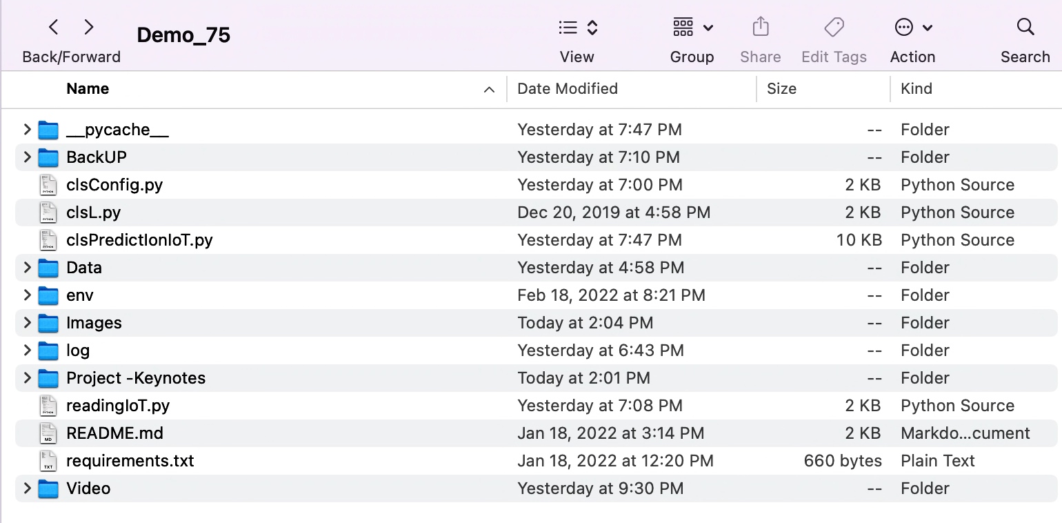
FOLDER STRUCTURE:

Here is the folder structure that contains all the files & directories in MAC O/S –

So, we’ve done it.

You will get the complete codebase in the following Github link.

If you want to know more about this legendary director & his famous work, please visit the following link.

I’ll bring some more exciting topic in the coming days from the Python verse. Please share & subscribe my post & let me know your feedback.

Till then, Happy Avenging! 😀

Note: All the data & scenario posted here are representational data & scenarios & available over the internet & for educational purpose only. Some of the images (except my photo) that we’ve used are available over the net. We don’t claim the ownership of these images. There is an always room for improvement & especially the prediction quality.