
I’ll bring an exciting streamlit app that will reflect the real-time dashboard by consuming all the events from the Ably channel.
One more time, I’ll be utilizing my IoT emulator that will feed the real-time events based on the user inputs to the Ably channel, which will be subscribed to by the Streamlit-based app.
However, I would like to share the run before we dig deep into this.
Isn’t this exciting? How we can use our custom-built IoT emulator & capture real-time events to Ably Queue, then transform those raw events into more meaningful KPIs? Let’s deep dive then.
Architecture:
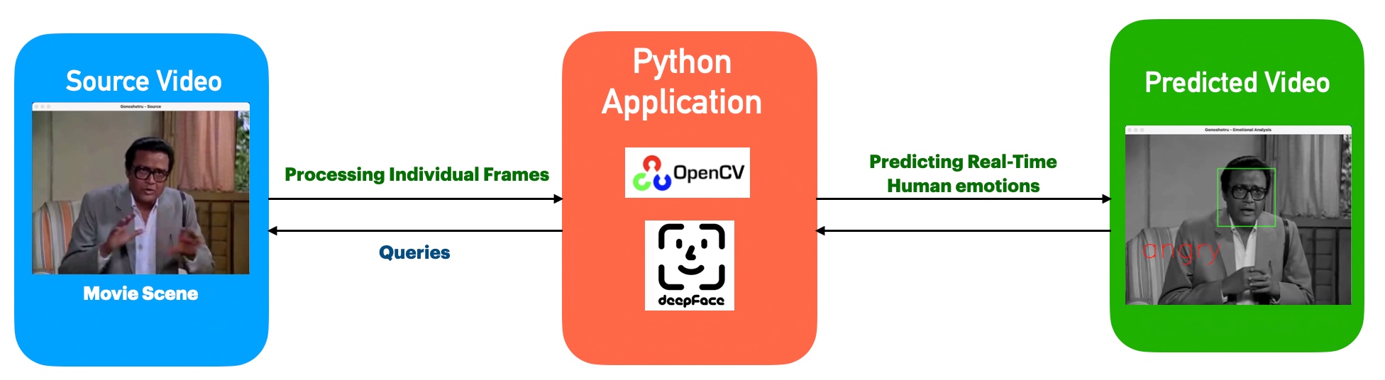
Let’s explore the broad-level architecture/flow –

As you can see, the green box is a demo IoT application that generates events & pushes them into the Ably Queue. At the same time, the streamlit-based Dashboard app consumes the events & transforms them into more meaningful metrics.
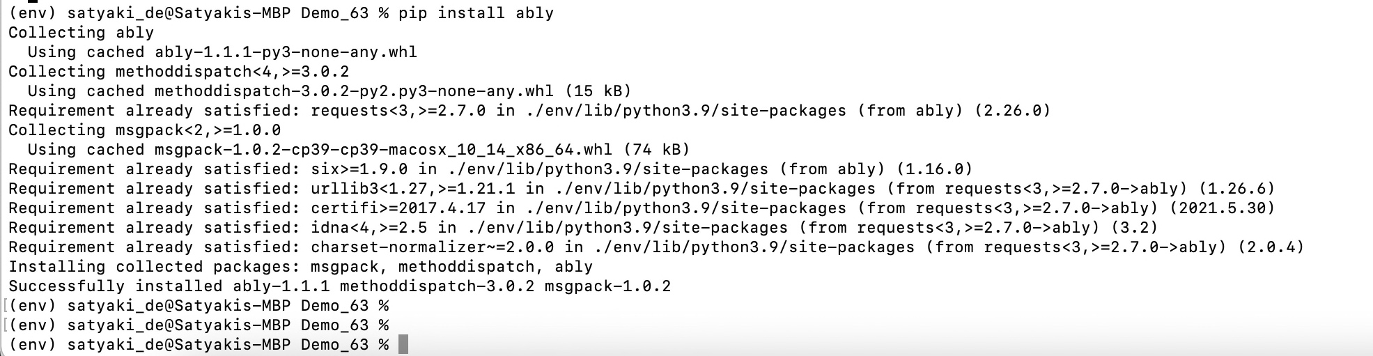
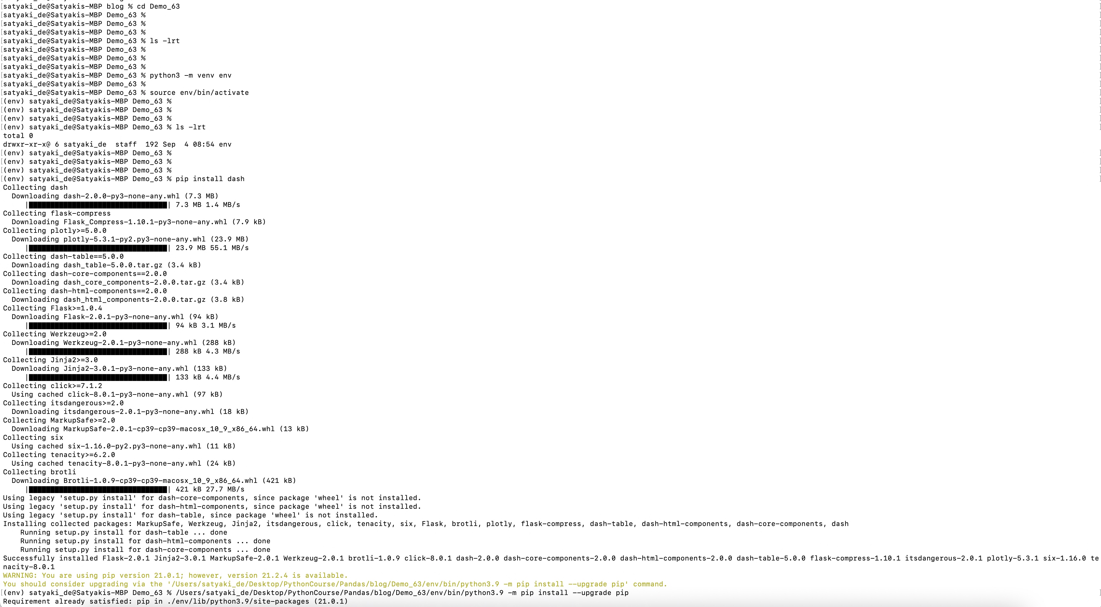
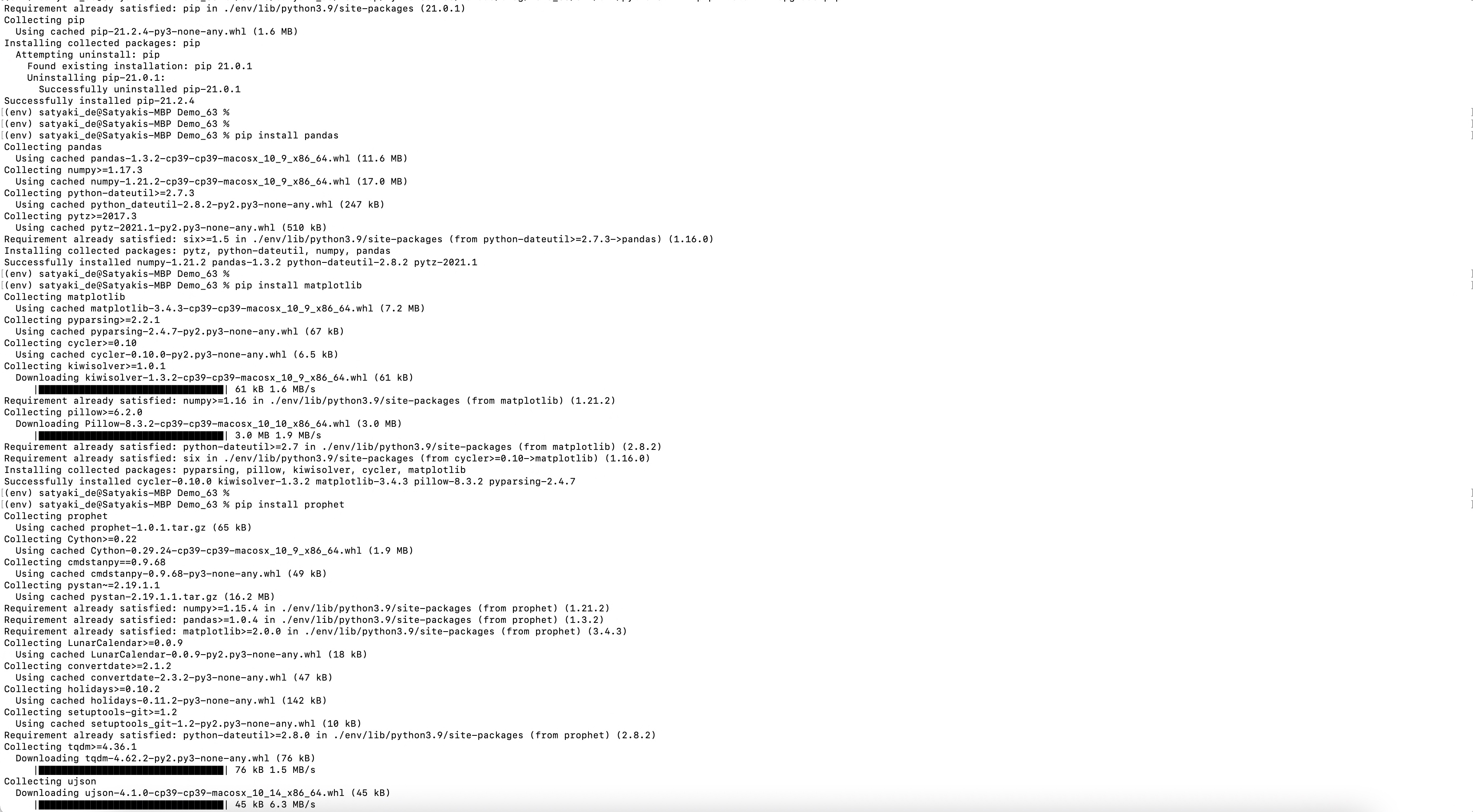
Package Installation:
Let us understand the sample packages that are required for this task.
pip install ably==2.0.3
pip install numpy==1.26.3
pip install pandas==2.2.0
pip install plotly==5.19.0
pip install requests==2.31.0
pip install streamlit==1.30.0
pip install streamlit-autorefresh==1.0.1
pip install streamlit-echarts==0.4.0
Code:
Since this is an extension to our previous post, we’re not going to discuss other scripts, which we’ve already discussed over there. Instead, we will talk about the enhanced scripts & the new scripts that are required for this use case.
1. app.py (This script will consume real-time streaming data coming out from a hosted API source using another popular third-party service named Ably. Ably mimics the pub sub-streaming concept, which might be extremely useful for any start-up. This will then translate into many meaningful KPIs in a streamlit-based dashboard app.)
Note that, we’re not going to discuss the entire script here. Only those parts are relevant. However, you can get the complete scripts in the GitHub repository.
def createHumidityGauge(humidity_value):
    fig = go.Figure(go.Indicator(
        mode = "gauge+number",
        value = humidity_value,
        domain = {'x': [0, 1], 'y': [0, 1]},
        title = {'text': "Humidity", 'font': {'size': 24}},
        gauge = {
            'axis': {'range': [None, 100], 'tickwidth': 1, 'tickcolor': "darkblue"},
            'bar': {'color': "darkblue"},
            'bgcolor': "white",
            'borderwidth': 2,
            'bordercolor': "gray",
            'steps': [
                {'range': [0, 50], 'color': 'cyan'},
                {'range': [50, 100], 'color': 'royalblue'}],
            'threshold': {
                'line': {'color': "red", 'width': 4},
                'thickness': 0.75,
                'value': humidity_value}
        }
    ))

    fig.update_layout(height=220, paper_bgcolor = "white", font = {'color': "darkblue", 'family': "Arial"}, margin=dict(t=0, l=5, r=5, b=0))

    return fig
The above function creates a customized humidity gauge that visually represents a given humidity value, making it easy to read and understand at a glance.
This code defines a function “createHumidityGauge“ that creates a visual gauge (like a meter) to display a humidity value. Here’s a simple breakdown of what it does:
- Function Definition: It starts by defining a function named
createHumidityGaugethat takes one parameter,humidity_value, which is the humidity level you want to display on the gauge. - Creating the Gauge: Inside the function, it creates a figure using Plotly (a plotting library) with a specific type of chart called an
Indicator. This Indicator is set to display in “gauge+number” mode, meaning it shows both a gauge visual and the numeric value of the humidity. - Setting Gauge Properties:
- The
valueis set to thehumidity_valueparameter, so the gauge shows this humidity level. - The
domainsets the position of the gauge on the plot, which is set to fill the available space ([0, 1] for both x and y axes). - The
titleis set to “Humidity” with a font size of 24, labeling the gauge. - The
gaugesection defines the appearance and behavior of the gauge, including:- An axis that goes from 0 to 100 (assuming humidity is measured as a percentage from 0% to 100%).
- The color and style of the gauge’s bar and background.
- Colored steps indicating different ranges of humidity (cyan for 0-50% and royal blue for 50-100%).
- A threshold line that appears at the value of the humidity, marked in red to stand out.
- The
- Finalizing the Gauge Appearance: The function then updates the layout of the figure to set its height, background color, font style, and margins to make sure the gauge looks nice and is visible.
- Returning the Figure: Finally, the function returns the
figobject, which is the fully configured gauge, ready to be displayed.
Other similar functions will repeat the same steps.
def createTemperatureLineChart(data):
    # Assuming 'data' is a DataFrame with a 'Timestamp' index and a 'Temperature' column
    fig = px.line(data, x=data.index, y='Temperature', title='Temperature Vs Time')
    fig.update_layout(height=270)  # Specify the desired height here
    return fig
The above function takes a set of temperature data indexed by timestamp and creates a line chart that visually represents how the temperature changes over time.
This code defines a function “createTemperatureLineChart” that creates a line chart to display temperature data over time. Here’s a simple summary of what it does:
- Function Definition: It starts with defining a function named “
createTemperatureLineChart“ that takes one parameter,data, which is expected to be a DataFrame (a type of data structure used in pandas, a Python data analysis library). This data frame should have a ‘Timestamp’ as its index (meaning each row represents a different point in time) and a ‘Temperature’ column containing temperature values. - Creating the Line Chart: The function uses Plotly Express (a plotting library) to create a line chart with the following characteristics:
- The x-axis represents time, taken from the DataFrame’s index (‘Timestamp’).
- The y-axis represents temperature, taken from the ‘Temperature’ column in the DataFrame.
- The chart is titled ‘Temperature Vs Time’, clearly indicating what the chart represents.
- Customizing the Chart: It then updates the layout of the chart to set a specific height (270 pixels) for the chart, making it easier to view.
- Returning the Chart: Finally, the function returns the
figobject, which is the fully prepared line chart, ready to be displayed.
Similar functions will repeat for other KPIs.
    st.sidebar.header("KPIs")
    selected_kpis = st.sidebar.multiselect(
        "Select KPIs", options=["Temperature", "Humidity", "Pressure"], default=["Temperature"]
    )
The above code will create a sidebar with drop-down lists, which will show the KPIs (“Temperature”, “Humidity”, “Pressure”).
# Split the layout into columns for KPIs and graphs
    gauge_col, kpi_col, graph_col = st.columns(3)

    # Auto-refresh setup
    st_autorefresh(interval=7000, key='data_refresh')

    # Fetching real-time data
    data = getData(var1, DInd)

    st.markdown(
        """
        <style>
        .stEcharts { margin-bottom: -50px; }  /* Class might differ, inspect the HTML to find the correct class name */
        </style>
        """,
        unsafe_allow_html=True
    )

    # Display gauges at the top of the page
    gauges = st.container()

    with gauges:
        col1, col2, col3 = st.columns(3)
        with col1:
            humidity_value = round(data['Humidity'].iloc[-1], 2)
            humidity_gauge_fig = createHumidityGauge(humidity_value)
            st.plotly_chart(humidity_gauge_fig, use_container_width=True)

        with col2:
            temp_value = round(data['Temperature'].iloc[-1], 2)
            temp_gauge_fig = createTempGauge(temp_value)
            st.plotly_chart(temp_gauge_fig, use_container_width=True)

        with col3:
            pressure_value = round(data['Pressure'].iloc[-1], 2)
            pressure_gauge_fig = createPressureGauge(pressure_value)
            st.plotly_chart(pressure_gauge_fig, use_container_width=True)


    # Next row for actual readings and charts side-by-side
    readings_charts = st.container()


    # Display KPIs and their trends
    with readings_charts:
        readings_col, graph_col = st.columns([1, 2])

        with readings_col:
            st.subheader("Latest Readings")
            if "Temperature" in selected_kpis:
                st.metric("Temperature", f"{temp_value:.2f}%")

            if "Humidity" in selected_kpis:
                st.metric("Humidity", f"{humidity_value:.2f}%")

            if "Pressure" in selected_kpis:
                st.metric("Pressure", f"{pressure_value:.2f}%")


        # Graph placeholders for each KPI
        with graph_col:
            if "Temperature" in selected_kpis:
                temperature_fig = createTemperatureLineChart(data.set_index("Timestamp"))

                # Display the Plotly chart in Streamlit with specified dimensions
                st.plotly_chart(temperature_fig, use_container_width=True)

            if "Humidity" in selected_kpis:
                humidity_fig = createHumidityLineChart(data.set_index("Timestamp"))

                # Display the Plotly chart in Streamlit with specified dimensions
                st.plotly_chart(humidity_fig, use_container_width=True)

            if "Pressure" in selected_kpis:
                pressure_fig = createPressureLineChart(data.set_index("Timestamp"))

                # Display the Plotly chart in Streamlit with specified dimensions
st.plotly_chart(pressure_fig, use_container_width=True)- The code begins by splitting the Streamlit web page layout into three columns to separately display Key Performance Indicators (KPIs), gauges, and graphs.
- It sets up an auto-refresh feature with a 7-second interval, ensuring the data displayed is regularly updated without manual refreshes.
- Real-time data is fetched using a function called
getData, which takes unspecified parametersvar1andDInd. - A CSS style is injected into the Streamlit page to adjust the margin of Echarts elements, which may be used to improve the visual layout of the page.
- A container for gauges is created at the top of the page, with three columns inside it dedicated to displaying humidity, temperature, and pressure gauges.
- Each gauge (humidity, temperature, and pressure) is created by rounding the last value from the fetched data to two decimal places and then visualized using respective functions that create Plotly gauge charts.
- Below the gauges, another container is set up for displaying the latest readings and their corresponding graphs in a side-by-side layout, using two columns.
- The left column under “Latest Readings” displays the latest values for selected KPIs (temperature, humidity, pressure) as metrics.
- In the right column, for each selected KPI, a line chart is created using data with timestamps as indices and displayed using Plotly charts, allowing for a visual trend analysis.
- This structured approach enables a dynamic and interactive dashboard within Streamlit, offering real-time insights into temperature, humidity, and pressure with both numeric metrics and graphical trends, optimized for regular data refreshes and user interactivity.
Run:
Let us understand some of the important screenshots of this application –


So, we’ve done it.
I’ll bring some more exciting topics in the coming days from the Python verse.
Till then, Happy Avenging! 🙂
Note: All the data & scenarios posted here are representational data & scenarios & available over the internet & for educational purposes only.
There is always room for improvement in this kind of model & the solution associated with it. I’ve shown the basic ways to achieve the same for educational purposes only.


You must be logged in to post a comment.