This site mainly deals with various use cases demonstrated using Python, Data Science, Cloud basics, SQL Server, Oracle, Teradata along with SQL & their implementation. Expecting yours active participation & time. This blog can be access from your TP, Tablet & mobile also. Please provide your feedback.
This is a continuation of my previous post, which can be found here.
Let us recap the key takaways from our previous post –
Enterprise AI, utilizing the Model Context Protocol (MCP), leverages an open standard that enables AI systems to securely and consistently access enterprise data and tools. MCP replaces brittle “N×M” integrations between models and systems with a standardized client–server pattern: an MCP host (e.g., IDE or chatbot) runs an MCP client that communicates with lightweight MCP servers, which wrap external systems via JSON-RPC. Servers expose three assets—Resources (data), Tools (actions), and Prompts (templates)—behind permissions, access control, and auditability. This design enables real-time context, reduces hallucinations, supports model- and cloud-agnostic interoperability, and accelerates “build once, integrate everywhere” deployment. A typical flow (e.g., retrieving a customer’s latest order) encompasses intent parsing, authorized tool invocation, query translation/execution, and the return of a normalized JSON result to the model for natural-language delivery. Performance introduces modest overhead (RPC hops, JSON (de)serialization, network transit) and scale considerations (request volume, significant results, context-window pressure). Mitigations include in-memory/semantic caching, optimized SQL with indexing, pagination, and filtering, connection pooling, and horizontal scaling with load balancing. In practice, small latency costs are often outweighed by the benefits of higher accuracy, stronger governance, and a decoupled, scalable architecture.
How does MCP compare with other AI integration approaches?
Compared to other approaches, the Model Context Protocol (MCP) offers a uniquely standardized and secure framework for AI-tool integration, shifting from brittle, custom-coded connections to a universal plug-and-play model. It is not a replacement for underlying systems, such as APIs or databases, but instead acts as an intelligent, secure abstraction layer designed explicitly for AI agents.
MCP vs. Custom API integrations:
This approach was the traditional method for AI integration before standards like MCP emerged.
Custom API integrations (traditional): Each AI application requires a custom-built connector for every external system it needs to access, leading to an N x M integration problem (the number of connectors grows exponentially with the number of models and systems). This approach is resource-intensive, challenging to maintain, and prone to breaking when underlying APIs change.
MCP: The standardized protocol eliminates the N x M problem by creating a universal interface. Tool creators build a single MCP server for their system, and any MCP-compatible AI agent can instantly access it. This process decouples the AI model from the underlying implementation details, drastically reducing integration and maintenance costs.
For more detailed information, please refer to the following link.
MCP vs. Retrieval-Augmented Generation (RAG):
RAG is a technique that retrieves static documents to augment an LLM’s knowledge, while MCP focuses on live interactions. They are complementary, not competing.
RAG:
Focus: Retrieving and summarizing static, unstructured data, such as documents, manuals, or knowledge bases.
Best for: Providing background knowledge and general information, as in a policy lookup tool or customer service bot.
Data type: Unstructured, static knowledge.
MCP:
Focus: Accessing and acting on real-time, structured, and dynamic data from databases, APIs, and business systems.
Best for: Agentic use cases involving real-world actions, like pulling live sales reports from a CRM or creating a ticket in a project management tool.
Data type: Structured, real-time, and dynamic data.
MCP vs. LLM plugins and extensions:
Before MCP, platforms like OpenAI offered proprietary plugin systems to extend LLM capabilities.
LLM plugins:
Proprietary: Tied to a specific AI vendor (e.g., OpenAI).
Limited: Rely on the vendor’s API function-calling mechanism, which focuses on call formatting but not standardized execution.
Centralized: Managed by the AI vendor, creating a risk of vendor lock-in.
MCP:
Open standard: Based on a public, interoperable protocol (JSON-RPC 2.0), making it model-agnostic and usable across different platforms.
Infrastructure layer: Provides a standardized infrastructure for agents to discover and use any compliant tool, regardless of the underlying LLM.
Decentralized: Promotes a flexible ecosystem and reduces the risk of vendor lock-in.
How enterprise AI with MCP has opened up a specific Architecture pattern for Azure, AWS & GCP?
Microsoft Azure:
The “agent factory” pattern: Azure focuses on providing managed services for building and orchestrating AI agents, tightly integrated with its enterprise security and governance features. The MCP architecture is a core component of the Azure AI Foundry, serving as a secure, managed “agent factory.”
Azure architecture pattern with MCP:
AI orchestration layer: The Azure AI Agent Service, within Azure AI Foundry, acts as the central host and orchestrator. It provides the control plane for creating, deploying, and managing multiple specialized agents, and it natively supports the MCP standard.
AI model layer: Agents in the Foundry can be powered by various models, including those from Azure OpenAI Service, commercial models from partners, or open-source models.
MCP server and tool layer: MCP servers are deployed using serverless functions, such as Azure Functions or Azure Logic Apps, to wrap existing enterprise systems. These servers expose tools for interacting with enterprise data sources like SharePoint, Azure AI Search, and Azure Blob Storage.
Data and security layer: Data is secured using Microsoft Entra ID (formerly Azure AD) for authentication and access control, with robust security policies enforced via Azure API Management. Access to data sources, such as databases and storage, is managed securely through private networks and Managed Identity.
Amazon Web Services (AWS):
The “composable serverless agent” pattern: AWS emphasizes a modular, composable, and serverless approach, leveraging its extensive portfolio of services to build sophisticated, flexible, and scalable AI solutions. The MCP architecture here aligns with the principle of creating lightweight, event-driven services that AI agents can orchestrate.
AWS architecture pattern with MCP:
The AI orchestration layer, which includesAmazon Bedrock Agents or custom agent frameworks deployed via AWS Fargate or Lambda, acts as the MCP hosts. Bedrock Agents provide built-in orchestration, while custom agents offer greater flexibility and customization options.
AI model layer: The models are sourced from Amazon Bedrock, which provides a wide selection of foundation models.
MCP server and tool layer: MCP servers are deployed as serverless AWS Lambda functions. AWS offers pre-built MCP servers for many of its services, including the AWS Serverless MCP Server for managing serverless applications and the AWS Lambda Tool MCP Server for invoking existing Lambda functions as tools.
Data and security layer: Access is tightly controlled using AWS Identity and Access Management (IAM) roles and policies, with fine-grained permissions for each MCP server. Private data sources like databases (Amazon DynamoDB) and storage (Amazon S3) are accessed securely within a Virtual Private Cloud (VPC).
Google Cloud Platform (GCP):
The “unified workbench” pattern: GCP focuses on providing a unified, open, and data-centric platform for AI development. The MCP architecture on GCP integrates natively with the Vertex AI platform, treating MCP servers as first-class tools that can be dynamically discovered and used within a single workbench.
GCP architecture pattern with MCP:
AI orchestration layer: The Vertex AI Agent Builder serves as the central environment for building and managing conversational AI and other agents. It orchestrates workflows and manages tool invocation for agents.
AI model layer: Agents use foundation models available through the Vertex AI Model Garden or the Gemini API.
MCP server and tool layer: MCP servers are deployed as containerized microservices on Cloud Run or managed by services like App Engine. These servers contain tools that interact with GCP services, such as BigQuery, Cloud Storage, and Cloud SQL. GCP offers pre-built MCP server implementations, such as the GCP MCP Toolbox, for integration with its databases.
Data and security layer:Vertex AI Vector Search and other data sources are encapsulated within the MCP server tools to provide contextual information. Access to these services is managed by Identity and Access Management (IAM) and secured through virtual private clouds. The MCP server can leverage Vertex AI Context Caching for improved performance.
Note that all the native technology is referred to in each respective cloud. Hence, some of the better technologies can be used in place of the tool mentioned here. This is more of a concept-level comparison rather than industry-wise implementation approaches.
We’ll go ahead and conclude this post here & continue discussing on a further deep dive in the next post.
Till then, Happy Avenging! 🙂
Note: All the data & scenarios posted here are representational data & scenarios & available over the internet & for educational purposes only. There is always room for improvement in this kind of model & the solution associated with it. I’ve shown the basic ways to achieve the same for educational purposes only.
Today, we’ll share the second installment of the RAG implementation. If you are new here, please visit the previous post for full context.
In this post, we’ll be discussing the Haystack framework more. Again, before discussing the main context, I want to present the demo here.
Demo
FLOW OF EVENTS:
Let us look at the flow diagram as it captures the sequence of events that unfold as part of the process, where today, we’ll pay our primary attention.
As you can see today, we’ll discuss the red dotted line, which contextualizes the source data into the Vector DBs.
Let us understand the flow of events here –
The main Python application will consume the nested JSON by invoking the museum API in multiple threads.
The application will clean the nested data & extract the relevant attributes after flattening the JSON.
It will create the unstructured text-based context, which is later fed to the Vector DB framework.
We’re using the Metropolitan Museum API to feed the data to our Vector DB. For more information, please visit the following link. And this is free to use & moreover, we’re using it for education scenarios.
CODE:
We’ll discuss the tokenization part highlighted in a red dotted line from the above picture.
Python:
We’ll discuss the scripts in the diagram as part of the flow mentioned above.
clsExtractJSON.py (This is the main class that will extract the content from the museum API using parallel calls.)
The above code translates into the following steps –
The above method first calls the generateFirstDayOfLastTenYears() plan to populate records for every department after getting all the unique departments by calling another API.
Then, it will call the getDataThread() methods to fetch all the relevant APIs simultaneously to reduce the overall wait time & create individual smaller files.
Finally, the application will invoke the mergeCsvFilesInDirectory() method to merge all the chunk files into one extensive historical data.
The above method will merge all the small files into a single, more extensive historical data that contains over ten years of data (the first day of ten years of data, to be precise).
For the complete code, please visit the GitHub.
1_ReadMuseumJSON.py (This is the main class that will invoke the class, which will extract the content from the museum API using parallel calls.)
The above script calls the main class after instantiating the class.
clsCreateList.py (This is the main class that will extract the relevant attributes from the historical files & then create the right input text to create the documents for contextualize into the Vector DB framework.)
The above code will read the data from the extensive historical file created from the earlier steps & then it will clean the file by removing all the duplicate records (if any) & finally, it will create three unique URLs that constitute artist, object & wiki.
Also, this application will remove the hyperlink with a specific hash value, which will feed into the vector DB. Vector DB could be better with the URLs. Hence, we will store the URLs in a separate file by storing the associate hash value & later, we’ll fetch it in a lookup from the open AI response.
Then, this application will generate prompts dynamically & finally create the documents for later steps of vector DB consumption by invoking the addDocument() methods.
For more details, please visit the GitHub link.
1_1_testCreateRec.py (This is the main class that will call the above class.)
In the above script, the following essential steps took place –
First, the application calls the clsCreateList class to store all the documents inside a dictionary.
Then it stores the data inside the vector DB & creates & stores the model, which will be later reused (If you remember, we’ve used this as a model in our previous post).
Finally, test with some sample use cases by providing the proper context to OpenAI & confirm the response.
Here is a short clip of how the RAG models contextualize with the source data.
RAG-ModelContextualization
So, finally, we’ve done it.
I know that this post is relatively bigger than my earlier post. But, I think, you can get all the details once you go through it.
You will get the complete codebase in the following GitHub link.
I’ll bring some more exciting topics in the coming days from the Python verse. Please share & subscribe to my post & let me know your feedback.
Till then, Happy Avenging! 🙂
Note: All the data & scenarios posted here are representational data & scenarios & available over the internet & for educational purposes only. Some of the images (except my photo) we’ve used are available over the net. We don’t claim ownership of these images. There is always room for improvement & especially in the prediction quality.
Today, I will share a new post in a part series about creating end-end LLMs that feed source data with RAG implementation. I’ll also use OpenAI python-based SDK and Haystack embeddings in this case.
In this post, I’ve directly subscribed to OpenAI & I’m not using OpenAI from Azure. However, I’ll explore that in the future as well.
Before I explain the process to invoke this new library, why not view the demo first & then discuss it?
Demo
FLOW OF EVENTS:
Let us look at the flow diagram as it captures the sequence of events that unfold as part of the process.
As you can see, to enable this large & complex solution, we must first establish the capabilities to build applications powered by LLMs, Transformer models, vector search, and more. You can use state-of-the-art NLP models to perform question-answering, answer generation, semantic document search, or build tools capable of complex decision-making and query resolution. Hence, steps no. 1 & 2 showcased the data embedding & creating that informed repository. We’ll be discussing that in our second part.
Once you have the informed repository, the system can interact with the end-users. As part of the query (shown in step 3), the prompt & the question are shared with the process engine, which then turned to reduce the volume & get relevant context from our informed repository & get the tuned context as part of the response (Shown in steps 4, 5 & 6).
Then, this tuned context is shared with the OpenAI for better response & summary & concluding remarks that are very user-friendly & easier to understand for end-users (Shown in steps 8 & 9).
IMPORTANT PACKAGES:
The following are the important packages that are essential to this project –
Let us understand some of the important sections of the above script –
Function – login():
The login function retrieves a ‘username’ and ‘password’ from a JSON request and prints them. It checks if the provided credentials are missing from users or password lists, returning a failure JSON response if so. It creates and returns an access token in a JSON response if valid.
Function – get_chat():
The get_chat function retrieves the running session count and user input from a JSON request. Based on the session count, it extracts catalog data or processes the user’s message from the RAG framework that finally receives the refined response from the OpenAI, extracting hash values, image URLs, and wiki URLs. If an error arises, the function captures and returns the error as a JSON message.
Function – updateCounter():
The updateCounter function checks if a given CSV file exists and retrieves its counter value. It then increments the counter and writes it back to the CSV. If any errors occur, an error message is printed, and the function returns a value of 1.
Function – extractRemoveUrls():
The extractRemoveUrls function attempts to filter a data frame, resDf, based on a provided hash value to extract image and wiki URLs. If the data frame contains matching entries, it retrieves the corresponding URLs. Any errors encountered are printed, but the function always returns the image and wiki URLs, even if they are empty.
clsContentScrapper.py (This is the main class that brings the default options for the users if they agree with the initial prompt by the bot.)
Let us understand the the core part that require from this class.
Function – extractCatalog():
The extractCatalog function uses specific headers to make a GET request to a constructed URL. The URL is derived by appending ‘/departments’ to a base_url, and a header token is used in the request headers. If successful, it returns the text of the response; if there’s an exception, it prints the error and returns the error message.
clsRAGOpenAI.py (This is the main class that brings the RAG-enabled context that is fed to OpenAI for fine-tuned response with less cost.)
############################################################# Written By:SATYAKIDE ######## Written On:27-Jun-2023 ######## ModifiedOn28-Jun-2023 ######## ######## Objective:Thisisthemaincalling ######## pythonscriptthatwillinvokethe ######## shortcutapplicationcreatedinsideMAC ######## enviornmentincludingMacBook,IPadorIPhone. ######## #############################################################fromhaystack.document_stores.faissimportFAISSDocumentStorefromhaystack.nodesimportDensePassageRetrieverimportopenaifromclsConfigClientimportclsConfigClientascfimportclsLaslog# DisblingWarningdefwarn(*args,**kwargs):passimportwarningswarnings.warn = warnimportosimportre################################################## GlobalSection ##################################################Ind = cf.conf['DEBUG_IND']queryModel = cf.conf['QUERY_MODEL']passageModel = cf.conf['PASSAGE_MODEL']#InitiatingLoggingInstancesclog = log.clsL()os.environ["TOKENIZERS_PARALLELISM"] = "false"vectorDBFileName = cf.conf['VECTORDB_FILE_NM']indexFile = "vectorDB/" + str(vectorDBFileName) + '.faiss'indexConfig = "vectorDB/" + str(vectorDBFileName) + ".json"print('File: ',str(indexFile))print('Config: ',str(indexConfig))# Also,provide`config_path`parameterifyousetitwhencallingthe`save()`method:new_document_store = FAISSDocumentStore.load(index_path=indexFile,config_path=indexConfig)# InitializeRetrieverretriever = DensePassageRetriever(document_store=new_document_store,query_embedding_model=queryModel,passage_embedding_model=passageModel,use_gpu=False)################################################## EndofGlobalSection ##################################################classclsRAGOpenAI:def__init__(self):self.basePath = cf.conf['DATA_PATH']self.fileName = cf.conf['FILE_NAME']self.Ind = cf.conf['DEBUG_IND']self.subdir = str(cf.conf['OUT_DIR'])self.base_url = cf.conf['BASE_URL']self.outputPath = cf.conf['OUTPUT_PATH']self.vectorDBPath = cf.conf['VECTORDB_PATH']self.openAIKey = cf.conf['OPEN_AI_KEY']self.temp = cf.conf['TEMP_VAL']self.modelName = cf.conf['MODEL_NAME']self.maxToken = cf.conf['MAX_TOKEN']defextractHash(self,text):try: # Regularexpressionpatterntomatch'Ref: {'followedbyanumberandthen'}'pattern = r"Ref: \{'(\d+)'\}"match = re.search(pattern,text)ifmatch:returnmatch.group(1)else:returnNoneexceptExceptionase:x = str(e)print('Error: ',x)returnNonedefremoveSentencesWithNaN(self,text):try: # Splittextintosentencesusingregularexpressionsentences = re.split('(?<!\w\.\w.)(?<![A-Z][a-z]\.)(?<=\.|\?)\s',text) # Filteroutsentencescontaining'nan'filteredSentences = [sentenceforsentenceinsentencesif'nan'notinsentence] # Rejointhesentencesreturn''.join(filteredSentences)exceptExceptionase:x = str(e)print('Error: ',x)return''defretrieveDocumentsReader(self,question,top_k=9):returnretriever.retrieve(question,top_k=top_k)defgenerateAnswerWithGPT3(self,retrieved_docs,question):try:openai.api_key = self.openAIKeytemp = self.tempmodelName = self.modelNamemaxToken = self.maxTokendocumentsText = "".join([doc.contentfordocinretrieved_docs])filteredDocs = self.removeSentencesWithNaN(documentsText)hashValue = self.extractHash(filteredDocs)print('RAG Docs:: ')print(filteredDocs) #prompt = f"Given the following documents: {documentsText}, answer the question accurately based on the above data with the supplied http urls: {question}" # Setupachat-stylepromptwithyourdatamessages = [{"role": "system", "content": "Youareahelpfulassistant,answerthequestionaccuratelybasedontheabovedatawiththesuppliedhttpurls. Onlyrelevantcontentneedstopublish. Pleasedonotprovidethefactsorthetextsthatresultscrossingthemax_tokenlimits."},{"role": "user", "content": filteredDocs} ] # Chatstyleinvokingthelatestmodelresponse = openai.ChatCompletion.create(model=modelName,messages=messages,temperature = temp,max_tokens=maxToken )returnhashValue,response.choices[0].message['content'].strip().replace('\n','\\n')exceptExceptionase:x = str(e)print('failed to get from OpenAI: ',x)return'Not Available!'defragAnswerWithHaystackAndGPT3(self,question):retrievedDocs = self.retrieveDocumentsReader(question)returnself.generateAnswerWithGPT3(retrievedDocs,question)defgetData(self,strVal):try:print('*'*120)print('Index Your Data for Retrieval:')print('*'*120)print('Response from New Docs: ')print()hashValue,answer = self.ragAnswerWithHaystackAndGPT3(strVal)print('GPT3 Answer::')print(answer)print('Hash Value:')print(str(hashValue))print('*'*240)print('End Of Use RAG to Generate Answers:')print('*'*240)returnhashValue,answerexceptExceptionase:x = str(e)print('Error: ',x)answer = xhashValue = 1returnhashValue,answer
Let us understand some of the important block –
Function – ragAnswerWithHaystackAndGPT3():
The ragAnswerWithHaystackAndGPT3 function retrieves relevant documents for a given question using the retrieveDocumentsReader method. It then generates an answer for the query using GPT-3 with the retrieved documents via the generateAnswerWithGPT3 method. The final response is returned.
Function – generateAnswerWithGPT3():
The generateAnswerWithGPT3 function, given a list of retrieved documents and a question, communicates with OpenAI’s GPT-3 to generate an answer. It first processes the documents, filtering and extracting a hash value. Using a chat-style format, it prompts GPT-3 with the processed documents and captures its response. If an error occurs, an error message is printed, and “Not Available!” is returned.
Function – retrieveDocumentsReader():
The retrieveDocumentsReader function takes in a question and an optional parameter, top_k (defaulted to 9). It is called the retriever.retrieve method with the given parameters. The result of the retrieval will generate at max nine responses from the RAG engine, which will be fed to OpenAI.
React:
App.js (This is the main react script, that will create the interface & parse the data apart from the authentication)
// App.jsimportReact,{useState}from'react';importaxiosfrom'axios';import'./App.css';constApp=()=>{const[isLoggedIn,setIsLoggedIn]=useState(false);const[username,setUsername]=useState('');const[password,setPassword]=useState('');const[message,setMessage]=useState('');const[chatLog,setChatLog]=useState([{sender:'MuBot',message:'Welcome to MuBot! Please explore the world of History from our brilliant collections! Do you want to proceed to see the catalog?'}]);consthandleLogin=async(e)=>{e.preventDefault();try{constresponse=awaitaxios.post('http://localhost:5000/login',{username,password});if (response.status===200) {setIsLoggedIn(true);}}catch (error) {console.error('Login error:',error);}};constsendMessage=async(username)=>{if (message.trim() ==='') return;// Create a new chat entryconstnewChatEntry={sender:'user',message:message.trim(),};// Clear the input fieldsetMessage('');try{// Make API request to Python-based APIconstresponse=awaitaxios.post('http://localhost:5000/chat',{message:newChatEntry.message});// Replace with your API endpoint URLconstresponseData=response.data;// Print the response to the console for debuggingconsole.log('API Response:',responseData);// Parse the nested JSON from the 'message' attributeconstjsonData=JSON.parse(responseData.message);// Check if the data contains 'departments'if (jsonData.departments) {// Extract the 'departments' attribute from the parsed dataconstdepartments=jsonData.departments;// Extract the department names and create a single string with line breaksconstbotResponseText=departments.reduce((acc,department)=>{returnacc+department.departmentId+''+department.displayName+'\n';},'');// Update the chat log with the bot's responsesetChatLog((prevChatLog)=> [...prevChatLog,{sender:'user',message:message},{sender:'bot',message:botResponseText},]);}elseif (jsonData.records){// Data structure 2: Artwork informationconstrecords=jsonData.records;// Prepare chat entriesconstchatEntries= [];// Iterate through records and extract text, image, and wiki informationrecords.forEach((record)=>{consttextInfo=Object.entries(record).map(([key,value])=>{if (key!=='Image'&&key!=='Wiki') {return`${key}: ${value}`;}returnnull;}).filter((info)=>info!==null).join('\n');constimageLink=record.Image;//const wikiLinks = JSON.parse(record.Wiki.replace(/'/g, '"'));//const wikiLinks = record.Wiki;constwikiLinks=record.Wiki.split(',').map(link=>link.trim());console.log('Wiki:',wikiLinks);// Check if there is a valid image linkconsthasValidImage=imageLink&&imageLink!=='[]';constimageElement=hasValidImage? (<imgsrc={imageLink}alt="Artwork"style={{maxWidth:'100%'}}/> ) :null;// Create JSX elements for rendering the wiki links (if available)constwikiElements=wikiLinks.map((link,index)=> (<divkey={index}><ahref={link}target="_blank"rel="noopener noreferrer"> Wiki Link {index+1}</a></div> ));if (textInfo) {chatEntries.push({sender:'bot',message:textInfo});}if (imageElement) {chatEntries.push({sender:'bot',message:imageElement});}if (wikiElements.length >0) {chatEntries.push({sender:'bot',message:wikiElements});}});// Update the chat log with the bot's responsesetChatLog((prevChatLog)=> [...prevChatLog,{sender:'user',message},...chatEntries, ]);}}catch (error) {console.error('Error sending message:',error);}};if (!isLoggedIn) {return (<divclassName="login-container"><h2>Welcome to the MuBot</h2><formonSubmit={handleLogin}className="login-form"><inputtype="text"placeholder="Enter your name"value={username}onChange={(e)=>setUsername(e.target.value)}required/><inputtype="password"placeholder="Enter your password"value={password}onChange={(e)=>setPassword(e.target.value)}required/><buttontype="submit">Login</button></form></div> );}return (<divclassName="chat-container"><divclassName="chat-header"><h2>Hello, {username}</h2><h3>Chat with MuBot</h3></div><divclassName="chat-log">{chatLog.map((chatEntry,index)=> (<divkey={index}className={`chat-entry ${chatEntry.sender==='user'?'user':'bot'}`}><spanclassName="user-name">{chatEntry.sender==='user'?username:'MuBot'}</span><pclassName="chat-message">{chatEntry.message}</p></div> ))}</div><divclassName="chat-input"><inputtype="text"placeholder="Type your message..."value={message}onChange={(e)=>setMessage(e.target.value)}onKeyPress={(e)=>{if (e.key==='Enter') {sendMessage();}}}/><buttononClick={sendMessage}>Send</button></div></div> );};exportdefaultApp;
Please find some of the important logic –
Function – handleLogin():
The handleLogin asynchronous function responds to an event by preventing its default action. It attempts to post a login request with a username and password to a local server endpoint. If the response is successful with a status of 200, it updates a state variable to indicate a successful login; otherwise, it logs any encountered errors.
Function – sendMessage():
The sendMessage asynchronous function is designed to handle the user’s chat interaction:
If the message is empty (after trimming spaces), the function exits without further action.
A chat entry object is created with the sender set as ‘user’ and the trimmed message.
The input field’s message is cleared, and an API request is made to a local server endpoint with the chat message.
If the API responds with a ‘departments’ attribute in its JSON, a bot response is crafted by iterating over department details.
If the API responds with ‘records’ indicating artwork information, the bot crafts responses for each record, extracting text, images, and wiki links, and generating JSX elements for rendering them.
After processing the API response, the chat log state is updated with the user’s original message and the bot’s responses.
Errors, if encountered, are logged to the console.
This function enables interactive chat with bot responses that vary based on the nature of the data received from the API.
DIRECTORY STRUCTURES:
Let us explore the directory structure starting from the parent to some of the important child folder should look like this –
So, finally, we’ve done it.
I know that this post is relatively bigger than my earlier post. But, I think, you can get all the details once you go through it.
You will get the complete codebase in the following GitHub link.
I’ll bring some more exciting topics in the coming days from the Python verse. Please share & subscribe to my post & let me know your feedback.
Till then, Happy Avenging! 🙂
Note: All the data & scenarios posted here are representational data & scenarios & available over the internet & for educational purposes only. Some of the images (except my photo) we’ve used are available over the net. We don’t claim ownership of these images. There is always room for improvement & especially in the prediction quality.
Today, I’ll discuss another important topic before I will share the excellent use case next month, as I still need some time to finish that one. We’ll see how we can leverage the brilliant capability of a low-code machine-learning library named PyCaret.
But before going through the details, why don’t we view the demo & then go through it?
Demo
Architecture:
Let us understand the flow of events –
As one can see, the initial training requests are triggered from the PyCaret-driven training models. And the application can successfully process & identify the best models out of the other combinations.
Python Packages:
Following are the python packages that are necessary to develop this use case –
pipinstallpandaspipinstallpycaret
PyCaret is dependent on a combination of other popular python packages. So, you need to install them successfully to run this package.
CODE:
clsConfigClient.py (Main configuration file)
This file contains hidden or bidirectional Unicode text that may be interpreted or compiled differently than what appears below. To review, open the file in an editor that reveals hidden Unicode characters. Learn more about bidirectional Unicode characters
I’m skipping this section as it is self-explanatory.
clsTrainModel.py (This is the main class that contains the core logic of low-code machine-learning library to evaluate the best model for your solutions.)
This file contains hidden or bidirectional Unicode text that may be interpreted or compiled differently than what appears below. To review, open the file in an editor that reveals hidden Unicode characters. Learn more about bidirectional Unicode characters
Import necessary libraries and load the Titanic dataset.
Initialize the PyCaret setup, specifying the target variable, train-test split, categorical and ordinal features, and features to ignore.
Compare various models to find the best-performing one.
Create a specific model (Random Forest in this case).
Perform hyper-parameter tuning on the Random Forest model.
Evaluate the model’s performance using a confusion matrix and AUC-ROC curve.
Finalize the model by training it on the complete dataset.
Make predictions on new data.
Save the trained model for future use.
trainPYCARETModel.py (This is the main calling python script that will invoke the training class of PyCaret package.)
This file contains hidden or bidirectional Unicode text that may be interpreted or compiled differently than what appears below. To review, open the file in an editor that reveals hidden Unicode characters. Learn more about bidirectional Unicode characters
The above code is pretty self-explanatory as well.
testPYCARETModel.py (This is the main calling python script that will invoke the testing script for PyCaret package.)
This file contains hidden or bidirectional Unicode text that may be interpreted or compiled differently than what appears below. To review, open the file in an editor that reveals hidden Unicode characters. Learn more about bidirectional Unicode characters
In this code, the application uses the stored model & then forecasts based on the optimized PyCaret model tuning.
Conclusion:
The above code demonstrates an end-to-end binary classification pipeline using the PyCaret library for the Titanic dataset. The goal is to predict whether a passenger survived based on the available features. Here are some conclusions you can draw from the code and data:
Ease of use: The code showcases how PyCaret simplifies the machine learning process, from data preprocessing to model training, evaluation, and deployment. With just a few lines of code, you can perform tasks that would require much more effort using lower-level libraries.
Model selection: The compare_models() function provides a quick and easy way to compare various machine learning algorithms and identify the best-performing one based on the chosen evaluation metric (accuracy by default). This selection helps you select a suitable model for the given problem.
Hyper-parameter tuning: The tune_model() function automates the process of hyper-parameter tuning to improve model performance. We tuned a Random Forest model to optimize its predictive power in the example.
Model evaluation: PyCaret provides several built-in visualization tools for assessing model performance. In the example, we used a confusion matrix and AUC-ROC curve to evaluate the performance of the tuned Random Forest model.
Model deployment: The example demonstrates how to make predictions using the trained model and save the model for future use. This deployment showcases how PyCaret can streamline the process of deploying a machine-learning model in a production environment.
It is important to note that the conclusions drawn from the code and data are specific to the Titanic dataset and the chosen features. Adjust the feature engineering, preprocessing, and model selection steps for different datasets or problems accordingly. However, the general workflow and benefits provided by PyCaret would remain the same.
So, finally, we’ve done it.
I know that this post is relatively bigger than my earlier post. But, I think, you can get all the details once you go through it.
You will get the complete codebase in the following GitHub link.
I’ll bring some more exciting topics in the coming days from the Python verse. Please share & subscribe to my post & let me know your feedback.
Till then, Happy Avenging! 🙂
Note: All the data & scenarios posted here are representational data & scenarios & available over the internet & for educational purposes only. Some of the images (except my photo) we’ve used are available over the net. We don’t claim ownership of these images. There is always room for improvement & especially in the prediction quality.
This week we’re going to extend one of our earlier posts & trying to read an entire text from streaming using computer vision. If you want to view the previous post, please click the following link.
But, before we proceed, why don’t we view the demo first?
Demo
Architecture:
Let us understand the architecture flow –
Architecture flow
The above diagram shows that the application, which uses the Open-CV, analyzes individual frames from the source & extracts the complete text within the video & displays it on top of the target screen besides prints the same in the console.
Let us now understand the code. For this use case, we will only discuss three python scripts. However, we need more than these three. However, we have already discussed them in some of the early posts. Hence, we will skip them here.
clsReadingTextFromStream.py (This is the main class of python script that will extract the text from the WebCAM streaming in real-time.)
This file contains hidden or bidirectional Unicode text that may be interpreted or compiled differently than what appears below. To review, open the file in an editor that reveals hidden Unicode characters. Learn more about bidirectional Unicode characters
Please find the key snippet from the above script –
# Two output layer names for the text detector model

lNames = cf.conf['LAYER_DET']

# Tesseract OCR text param values

strVal = "-l " + str(cf.conf['LANG']) + " --oem " + str(cf.conf['OEM_VAL']) + " --psm " + str(cf.conf['PSM_VAL']) + ""
config = (strVal)
The first line contains the two output layers’ names for the text detector model. Among them, the first one indicates the outcome possibilities & the second one use to derive the bounding box coordinates of the predicted text.
The second line contains various options for the tesseract APIs. You need to understand the opportunities in detail to make them work. These are the essential options for our use case –
Language – The intended language, for example, English, Spanish, Hindi, Bengali, etc.
OEM flag – In this case, the application will use 4 to indicate LSTM neural net model for OCR.
OEM Value – In this case, the selected value is 7, indicating that the application treats the ROI as a single line of text.
For more details, please refer to the config file.
print("[INFO] Loading Text Detector...")
net = cv2.dnn.readNet(modelPath)
The above lines bring the already created model & load it to memory for evaluation.
# Setting new width and height and then determine the ratio in change
# for both the width and height
(newW, newH) = (wt, ht)
rW = origW / float(newW)
rH = origH / float(newH)

# Resize the frame and grab the new frame dimensions
frame = cv2.resize(frame, (newW, newH))
(H, W) = frame.shape[:2]

# Construct a blob from the frame and then perform a forward pass of
# the model to obtain the two output layer sets
blob = cv2.dnn.blobFromImage(frame, 1.0, (W, H), sParam, swapRB=True, crop=False)
net.setInput(blob)
(confScore, imgGeo) = net.forward(lNames)

# Decode the predictions, then apply non-maxima suppression to
# suppress weak, overlapping bounding boxes
(rects, confidences) = self.predictText(confScore, imgGeo)
boxes = non_max_suppression(np.array(rects), probs=confidences)
The above lines are more of preparing individual frames to get the bounding box by resizing the height & width followed by a forward pass of the model to obtain two output layer sets. And then apply the non-maxima suppression to remove the weak, overlapping bounding box by interpreting the prediction. In short, this will identify the potential text region & put the bounding box surrounding it.
# Initialize the list of results
res = []

# Getting BoundingBox boundaries
res = self.findBoundBox(boxes, res, rW, rH, orig, origW, origH, pad)
The above function will create the bounding box surrounding the predicted text regions. Also, we will capture the expected text inside the result variable.
for (spX, spY, epX, epY) in boxes:
  # Scale the bounding box coordinates based on the respective
  # ratios
  spX = int(spX * rW)
  spY = int(spY * rH)
  epX = int(epX * rW)
  epY = int(epY * rH)

  # To obtain a better OCR of the text we can potentially
  # apply a bit of padding surrounding the bounding box.
  # And, computing the deltas in both the x and y directions
  dX = int((epX - spX) * pad)
  dY = int((epY - spY) * pad)

  # Apply padding to each side of the bounding box, respectively
  spX = max(0, spX - dX)
  spY = max(0, spY - dY)
  epX = min(origW, epX + (dX * 2))
  epY = min(origH, epY + (dY * 2))

  # Extract the actual padded ROI
  roi = orig[spY:epY, spX:epX]
Now, the application will scale the bounding boxes based on the previously computed ratio for actual text recognition. In this process, the application also padded the bounding boxes & then extracted the padded region of interest.
# Choose the proper OCR Config
text = pytesseract.image_to_string(roi, config=config)

# Add the bounding box coordinates and OCR'd text to the list
# of results
res.append(((spX, spY, epX, epY), text))
Using OCR options, the application extracts the text within the video frame & adds that to the res list.
# Sort the results bounding box coordinates from top to bottom
res = sorted(res, key=lambda r:r[0][1])
It then sends a sorted output to the primary calling functions.
for ((spX, spY, epX, epY), text) in res:
  # Display the text OCR by using Tesseract APIs
  print("Reading Text::")
  print("=" *60)
  print(text)
  print("=" *60)

  # Removing the non-ASCII text so it can draw the text on the frame
  # using OpenCV, then draw the text and a bounding box surrounding
  # the text region of the input frame
  text = "".join([c if ord(c) < aRange else "" for c in text]).strip()
  output = orig.copy()

  cv2.rectangle(output, (spX, spY), (epX, epY), drawTag, 2)
  cv2.putText(output, text, (spX, spY - 20), cv2.FONT_HERSHEY_SIMPLEX, 1.2, drawTag, 3)

  # Show the output frame
  cv2.imshow(title, output)
Finally, it fetches the potential text region along with the text & then prints on top of the source video. Also, it removed some non-printable characters during this time to avoid any cryptic texts.
readingVideo.py (Main calling script.)
This file contains hidden or bidirectional Unicode text that may be interpreted or compiled differently than what appears below. To review, open the file in an editor that reveals hidden Unicode characters. Learn more about bidirectional Unicode characters
# Instantiating all the main class

x1 = rtfs.clsReadingTextFromStream()

# Execute all the pass
r1 = x1.processStream(debugInd, var)

if (r1 == 0):
    print('Successfully read text from the Live Stream!')
else:
    print('Failed to read text from the Live Stream!')
The above lines instantiate the main calling class & then invoke the function to get the desired extracted text from the live streaming video if that is successful.
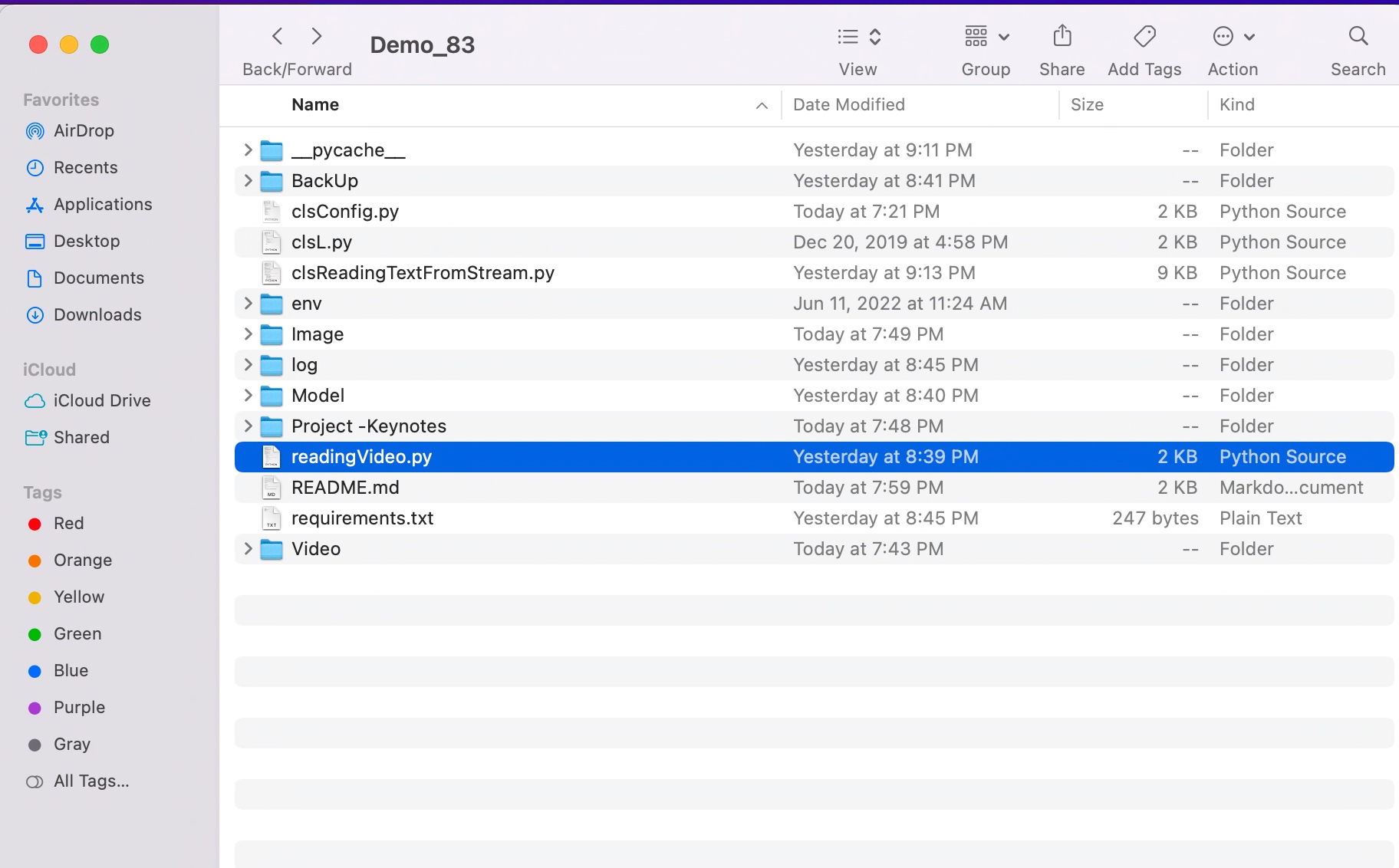
FOLDER STRUCTURE:
Here is the folder structure that contains all the files & directories in MAC O/S –
You will get the complete codebase in the following Github link.
Unfortunately, I cannot upload the model due to it’s size. I will share on the need basis.
I’ll bring some more exciting topic in the coming days from the Python verse. Please share & subscribe my post & let me know your feedback.
Till then, Happy Avenging! 🙂
Note: All the data & scenario posted here are representational data & scenarios & available over the internet & for educational purpose only. Some of the images (except my photo) that we’ve used are available over the net. We don’t claim the ownership of these images. There is an always room for improvement & especially the prediction quality.
This week we’re planning to touch on one of the exciting posts of visually reading characters from WebCAM & predict the letters using CNN methods. Before we dig deep, why don’t we see the demo run first?
Demo
Isn’t it fascinating? As we can see, the computer can record events and read like humans. And, thanks to the brilliant packages available in Python, which can help us predict the correct letter out of an Image.
What do we need to test it out?
Preferably an external WebCAM.
A moderate or good Laptop to test out this.
Python
And a few other packages that we’ll mention next block.
What Python packages do we need?
Some of the critical packages that we must need to test out this application are –
In deep learning, a convolutional neural network (CNN/ConvNet) is a class of deep neural networks most commonly applied to analyze visual imagery.
Different Steps of CNN
We can understand from the above picture that a CNN generally takes an image as input. The neural network analyzes each pixel separately. The weights and biases of the model are then tweaked to detect the desired letters (In our use case) from the image. Like other algorithms, the data also has to pass through pre-processing stage. However, a CNN needs relatively less pre-processing than most other Deep Learning algorithms.
If you want to know more about this, there is an excellent article on CNN with some on-point animations explaining this concept. Please read it here.
Where do we get the data sets for our testing?
For testing, we are fortunate enough to have Kaggle with us. We have received a wide variety of sample data, which you can get from here.
Our use-case:
Architecture
From the above diagram, one can see that the python application will consume a live video feed of any random letters (both printed & handwritten) & predict the character as part of the machine learning model that we trained.
Code:
clsConfig.py (Configuration file for the entire application.)
This file contains hidden or bidirectional Unicode text that may be interpreted or compiled differently than what appears below. To review, open the file in an editor that reveals hidden Unicode characters. Learn more about bidirectional Unicode characters
Since we have 26 letters, we have classified it as 26 in the numOfClasses.
Since we are talking about characters, we had to come up with a process of identifying each character as numbers & then processing our entire logic. Hence, the above parameter named word_dict captured all the characters in a python dictionary & stored them. Moreover, the application translates the final number output to more appropriate characters as the prediction.
2. clsAlphabetReading.py (Main training class to teach the model to predict alphabets from visual reader.)
This file contains hidden or bidirectional Unicode text that may be interpreted or compiled differently than what appears below. To review, open the file in an editor that reveals hidden Unicode characters. Learn more about bidirectional Unicode characters
We are splitting the data into Train, Test & Validation sets to get more accurate predictions and reshaping the raw data into the image by consuming the 784 data columns to 28×28 pixel images.
Since we are talking about characters, we had to come up with a process of identifying The following snippet will plot the character equivalent number into a matplotlib chart & showcase the overall distribution trend after splitting.
Y_Train_Num = np.int0(y)
count = np.zeros(numOfClasses, dtype='int')
for i in Y_Train_Num:
    count[i] +=1

alphabets = []
for i in word_dict.values():
    alphabets.append(i)

fig, ax = plt.subplots(1,1, figsize=(7,7))
ax.barh(alphabets, count)

plt.xlabel("Number of elements ")
plt.ylabel("Alphabets")
plt.grid()
plt.show(block=False)
plt.pause(sleepTime)
plt.close()
Note that we have tweaked the plt.show property with (block=False). This property will enable us to continue execution without human interventions after the initial pause.
# Model reshaping the training & test dataset
X_Train = X_Train.reshape(X_Train.shape[0],X_Train.shape[1],X_Train.shape[2],1)
print("Shape of Train Data: ", X_Train.shape)

X_Test = X_Test.reshape(X_Test.shape[0], X_Test.shape[1], X_Test.shape[2],1)
print("Shape of Test Data: ", X_Test.shape)

X_Validation = X_Validation.reshape(X_Validation.shape[0], X_Validation.shape[1], X_Validation.shape[2],1)
print("Shape of Validation data: ", X_Validation.shape)

# Converting the labels to categorical values
Y_Train_Catg = to_categorical(Y_Train, num_classes = numOfClasses, dtype='int')
print("Shape of Train Labels: ", Y_Train_Catg.shape)

Y_Test_Catg = to_categorical(Y_Test, num_classes = numOfClasses, dtype='int')
print("Shape of Test Labels: ", Y_Test_Catg.shape)

Y_Validation_Catg = to_categorical(Y_Validation, num_classes = numOfClasses, dtype='int')
print("Shape of validation labels: ", Y_Validation_Catg.shape)
In the above diagram, the application did reshape all three categories of data before calling the primary CNN function.
In the above snippet, the convolution layers are followed by maxpool layers, which reduce the number of features extracted. The output of the maxpool layers and convolution layers are flattened into a vector of a single dimension and supplied as an input to the Dense layer—the CNN model prepared for training the model using the training dataset.
We have used optimization parameters like Adam, RMSProp & the application we trained for eight epochs for better accuracy & predictions.
# Displaying the accuracies & losses for train & validation set
print("Validation Accuracy :", history.history['val_accuracy'])
print("Training Accuracy :", history.history['accuracy'])
print("Validation Loss :", history.history['val_loss'])
print("Training Loss :", history.history['loss'])

# Displaying the Loss Graph
plt.figure(1)
plt.plot(history.history['loss'])
plt.plot(history.history['val_loss'])
plt.legend(['training','validation'])
plt.title('Loss')
plt.xlabel('epoch')
plt.show(block=False)
plt.pause(sleepTime1)
plt.close()

# Dsiplaying the Accuracy Graph
plt.figure(2)
plt.plot(history.history['accuracy'])
plt.plot(history.history['val_accuracy'])
plt.legend(['training','validation'])
plt.title('Accuracy')
plt.xlabel('epoch')
plt.show(block=False)
plt.pause(sleepTime1)
plt.close()
Also, we have captured the validation Accuracy & Loss & plot them into two separate graphs for better understanding.
Also, the application is trying to get the accuracy of the model that we trained & validated with the training & validation data. This time we have used test data to predict the confidence score.
# Displaying some of the test images & their predicted labels
fig, ax = plt.subplots(3,3, figsize=(8,9))
axes = ax.flatten()

for i in range(9):
    axes[i].imshow(np.reshape(X_Test[i], reshapeVal1), cmap="Greys")
    pred = word_dict[np.argmax(Y_Test_Catg[i])]
    print('Prediction: ', pred)
    axes[i].set_title("Test Prediction: " + pred)
    axes[i].grid()
plt.show(block=False)
plt.pause(sleepTime1)
plt.close()
Finally, the application testing with some random test data & tried to plot the output & prediction assessment.
As a part of the last step, the application will generate the models using a pickle package & save them under a specific location, which the reader application will use.
3. trainingVisualDataRead.py (Main application that will invoke the training class to predict alphabet through WebCam using Convolutional Neural Network (CNN).)
This file contains hidden or bidirectional Unicode text that may be interpreted or compiled differently than what appears below. To review, open the file in an editor that reveals hidden Unicode characters. Learn more about bidirectional Unicode characters
The python application will invoke the class & capture the returned value inside the r1 variable.
4. readingVisualData.py (Reading the model to predict Alphabet using WebCAM.)
This file contains hidden or bidirectional Unicode text that may be interpreted or compiled differently than what appears below. To review, open the file in an editor that reveals hidden Unicode characters. Learn more about bidirectional Unicode characters
We have initially cloned the original video frame & then it converted from BGR2GRAYSCALE while applying the threshold on it doe better prediction outcomes. Then the image has resized & reshaped for model input. Finally, the np.argmax function extracted the class index with the highest predicted probability. Furthermore, it is translated using the word_dict dictionary to an Alphabet & displayed on top of the Live View.
Also, derive the confidence score of that probability & display that on top of the Live View.
if cv2.waitKey(1) & 0xFF == ord('q'):
    r1=0
    break
The above code will let the developer exit from this application by pressing the “Esc” or “q”-key from the keyboard & the program will terminate.
So, we’ve done it.
You will get the complete codebase in the following Github link.
I’ll bring some more exciting topic in the coming days from the Python verse. Please share & subscribe my post & let me know your feedback.
Till then, Happy Avenging! 😀
Note: All the data & scenario posted here are representational data & scenarios & available over the internet & for educational purpose only. Some of the images (except my photo) that we’ve used are available over the net. We don’t claim the ownership of these images. There is an always room for improvement & especially the prediction quality of Alphabet.
Today, I’ll be demonstrating a short but significant topic. There are widespread facts that, on many occasions, Python is relatively slower than other strongly typed programming languages like C++, Java, or even the latest version of PHP.
I found a relatively old post with a comparison shown between Python and the other popular languages. You can find the details at this link.
However, I haven’t verified the outcome. So, I can’t comment on the final statistics provided on that link.
My purpose is to find cases where I can take certain tricks to improve performance drastically.
One preferable option would be the use of Cython. That involves the middle ground between C & Python & brings the best out of both worlds.
The other option would be the use of GPU for vector computations. That would drastically increase the processing power. Today, we’ll be exploring this option.
Let’s find out what we need to prepare our environment before we try out on this.
Step – 1 (Installing dependent packages):
pip install pyopencl
pip install plaidml-keras
So, we will be taking advantage of the Keras package to use our GPU. And, the screen should look like this –
Installation Process of Python-based Packages
Once we’ve installed the packages, we’ll configure the package showing on the next screen.
Configuration of Packages
For our case, we need to install pandas as we’ll be using numpy, which comes default with it.
Installation of supplemental packages
Let’s explore our standard snippet to test this use case.
Case 1 (Normal computational code in Python):
##############################################
#### Written By: SATYAKI DE               ####
#### Written On: 18-Jan-2020              ####
####                                      ####
#### Objective: Main calling scripts for  ####
#### normal execution.                    ####
##############################################

import numpy as np
from timeit import default_timer as timer

def pow(a, b, c):
    for i in range(a.size):
         c[i] = a[i] ** b[i]

def main():
    vec_size = 100000000

    a = b = np.array(np.random.sample(vec_size), dtype=np.float32)
    c = np.zeros(vec_size, dtype=np.float32)

    start = timer()
    pow(a, b, c)
    duration = timer() - start

    print(duration)

if __name__ == '__main__':
    main()
Case 2 (GPU-based computational code in Python):
#################################################
#### Written By: SATYAKI DE                  ####
#### Written On: 18-Jan-2020                 ####
####                                         ####
#### Objective: Main calling scripts for     ####
#### use of GPU to speed-up the performance. ####
#################################################

import numpy as np
from timeit import default_timer as timer

# Adding GPU Instance
from os import environ
environ["KERAS_BACKEND"] = "plaidml.keras.backend"

def pow(a, b):
    return a ** b

def main():
    vec_size = 100000000

    a = b = np.array(np.random.sample(vec_size), dtype=np.float32)
    c = np.zeros(vec_size, dtype=np.float32)

    start = timer()
    c = pow(a, b)
    duration = timer() - start

    print(duration)

if __name__ == '__main__':
    main()
And, here comes the output for your comparisons –
Case 1 Vs Case 2:
Performance Comparisons
As you can see, there is a significant improvement that we can achieve using this. However, it has limited scope. Not everywhere you get the benefits. Until or unless Python decides to work on the performance side, you better need to explore either of the two options that I’ve discussed here (I didn’t mention a lot on Cython here. Maybe some other day.).
To get the codebase you can refer the following Github link.
So, finally, we have done it.
I’ll bring some more exciting topic in the coming days from the Python verse.
Till then, Happy Avenging! 😀
Note: All the data & scenario posted here are representational data & scenarios & available over the internet & for educational purpose only.


You must be logged in to post a comment.