|
############################################## |
|
#### Written By: SATYAKI DE #### |
|
#### Written On: 26-Jul-2021 #### |
|
#### Modified On 26-Jul-2021 #### |
|
#### #### |
|
#### Objective: Calling multiple API's #### |
|
#### that including Prophet-API developed #### |
|
#### by Facebook for future prediction of #### |
|
#### Covid-19 situations in upcoming days #### |
|
#### for world's major hotspots. #### |
|
############################################## |
|
|
|
import json |
|
|
|
import clsCovidAPI as ca |
|
from clsConfig import clsConfig as cf |
|
import datetime |
|
import logging |
|
import clsL as cl |
|
import math as m |
|
import clsPublishStream as cps |
|
|
|
import clsForecast as f |
|
|
|
from prophet import Prophet |
|
|
|
from prophet.plot import plot_plotly, plot_components_plotly |
|
|
|
import matplotlib.pyplot as plt |
|
import pandas as p |
|
import datetime as dt |
|
|
|
import time |
|
|
|
# Disbling Warning |
|
def warn(*args, **kwargs): |
|
pass |
|
|
|
import warnings |
|
warnings.warn = warn |
|
|
|
# Initiating Log class |
|
l = cl.clsL() |
|
|
|
# Helper Function that removes underscores |
|
def countryDet(inputCD): |
|
try: |
|
countryCD = inputCD |
|
|
|
if str(countryCD) == 'DE': |
|
cntCD = 'Germany' |
|
elif str(countryCD) == 'BR': |
|
cntCD = 'Brazil' |
|
elif str(countryCD) == 'GB': |
|
cntCD = 'UnitedKingdom' |
|
elif str(countryCD) == 'US': |
|
cntCD = 'UnitedStates' |
|
elif str(countryCD) == 'IN': |
|
cntCD = 'India' |
|
elif str(countryCD) == 'CA': |
|
cntCD = 'Canada' |
|
elif str(countryCD) == 'ID': |
|
cntCD = 'Indonesia' |
|
else: |
|
cntCD = 'N/A' |
|
|
|
return cntCD |
|
except: |
|
cntCD = 'N/A' |
|
|
|
return cntCD |
|
|
|
def lookupCountry(row): |
|
try: |
|
strCD = str(row['CountryCode']) |
|
|
|
retVal = countryDet(strCD) |
|
|
|
return retVal |
|
except: |
|
retVal = 'N/A' |
|
|
|
return retVal |
|
|
|
def adjustTrend(row): |
|
try: |
|
flTrend = float(row['trend']) |
|
flTrendUpr = float(row['trend_upper']) |
|
flTrendLwr = float(row['trend_lower']) |
|
|
|
retVal = m.trunc((flTrend + flTrendUpr + flTrendLwr)/3) |
|
|
|
if retVal < 0: |
|
retVal = 0 |
|
|
|
return retVal |
|
except: |
|
retVal = 0 |
|
|
|
return retVal |
|
|
|
def ceilTrend(row, colName): |
|
try: |
|
flTrend = str(row[colName]) |
|
|
|
if flTrend.find('.'): |
|
if float(flTrend) > 0: |
|
retVal = m.trunc(float(flTrend)) + 1 |
|
else: |
|
retVal = m.trunc(float(flTrend)) |
|
else: |
|
retVal = float(flTrend) |
|
|
|
if retVal < 0: |
|
retVal = 0 |
|
|
|
return retVal |
|
except: |
|
retVal = 0 |
|
|
|
return retVal |
|
|
|
def plot_picture(inputDF, debug_ind, var, countryCD, stat): |
|
try: |
|
iDF = inputDF |
|
|
|
# Lowercase the column names |
|
iDF.columns = [c.lower() for c in iDF.columns] |
|
# Determine which is Y axis |
|
y_col = [c for c in iDF.columns if c.startswith('y')][0] |
|
# Determine which is X axis |
|
x_col = [c for c in iDF.columns if c.startswith('ds')][0] |
|
|
|
# Data Conversion |
|
iDF['y'] = iDF[y_col].astype('float') |
|
iDF['ds'] = iDF[x_col].astype('datetime64[ns]') |
|
|
|
# Forecast calculations |
|
# Decreasing the changepoint_prior_scale to 0.001 to make the trend less flexible |
|
m = Prophet(n_changepoints=20, yearly_seasonality=True, changepoint_prior_scale=0.001) |
|
#m = Prophet(n_changepoints=20, yearly_seasonality=True, changepoint_prior_scale=0.04525) |
|
#m = Prophet(n_changepoints=['2021-09-10']) |
|
m.fit(iDF) |
|
|
|
forecastDF = m.make_future_dataframe(periods=365) |
|
|
|
forecastDF = m.predict(forecastDF) |
|
|
|
l.logr('15.forecastDF_' + var + '_' + countryCD + '.csv', debug_ind, forecastDF, 'log') |
|
|
|
df_M = forecastDF[['ds', 'trend', 'trend_lower', 'trend_upper']] |
|
|
|
l.logr('16.df_M_' + var + '_' + countryCD + '.csv', debug_ind, df_M, 'log') |
|
|
|
# Getting Full Country Name |
|
cntCD = countryDet(countryCD) |
|
|
|
# Draw forecast results |
|
df_M['Country'] = cntCD |
|
|
|
l.logr('17.df_M_C_' + var + '_' + countryCD + '.csv', debug_ind, df_M, 'log') |
|
|
|
df_M['AdjustTrend'] = df_M.apply(lambda row: adjustTrend(row), axis=1) |
|
|
|
l.logr('20.df_M_AdjustTrend_' + var + '_' + countryCD + '.csv', debug_ind, df_M, 'log') |
|
|
|
return df_M |
|
|
|
except Exception as e: |
|
x = str(e) |
|
print(x) |
|
|
|
df = p.DataFrame() |
|
|
|
return df |
|
|
|
def countrySpecificDF(counryDF, val): |
|
try: |
|
countryName = val |
|
df = counryDF |
|
|
|
df_lkpFile = df[(df['CountryCode'] == val)] |
|
|
|
return df_lkpFile |
|
except: |
|
df = p.DataFrame() |
|
|
|
return df |
|
|
|
def toNum(row, colName): |
|
try: |
|
flTrend = str(row[colName]) |
|
flTr, subpart = flTrend.split(' ') |
|
retVal = int(flTr.replace('-','')) |
|
|
|
return retVal |
|
except: |
|
retVal = 0 |
|
|
|
return retVal |
|
|
|
def extractPredictedDF(OrigDF, MergePredictedDF, colName): |
|
try: |
|
iDF_1 = OrigDF |
|
iDF_2 = MergePredictedDF |
|
|
|
dt_format = '%Y-%m-%d' |
|
|
|
iDF_1_max_group = iDF_1.groupby(["Country"] , as_index=False)["ReportedDate"].max() |
|
|
|
iDF_2['ReportedDate'] = iDF_2.apply(lambda row: toNum(row, 'ds'), axis=1) |
|
|
|
col_one_list = iDF_1_max_group['Country'].tolist() |
|
col_two_list = iDF_1_max_group['ReportedDate'].tolist() |
|
|
|
print('col_one_list: ', str(col_one_list)) |
|
print('col_two_list: ', str(col_two_list)) |
|
|
|
cnt_1_x = 1 |
|
cnt_1_y = 1 |
|
cnt_x = 0 |
|
|
|
df_M = p.DataFrame() |
|
|
|
for i in col_one_list: |
|
str_countryVal = str(i) |
|
cnt_1_y = 1 |
|
|
|
for j in col_two_list: |
|
|
|
intReportDate = int(str(j).strip().replace('-','')) |
|
|
|
if cnt_1_x == cnt_1_y: |
|
print('str_countryVal: ', str(str_countryVal)) |
|
print('intReportDate: ', str(intReportDate)) |
|
|
|
iDF_2_M = iDF_2[(iDF_2['Country'] == str_countryVal) & (iDF_2['ReportedDate'] > intReportDate)] |
|
|
|
# Merging with the previous Country Code data |
|
if cnt_x == 0: |
|
df_M = iDF_2_M |
|
else: |
|
d_frames = [df_M, iDF_2_M] |
|
df_M = p.concat(d_frames) |
|
|
|
cnt_x += 1 |
|
|
|
cnt_1_y += 1 |
|
|
|
cnt_1_x += 1 |
|
|
|
df_M.drop(columns=['ReportedDate'], axis=1, inplace=True) |
|
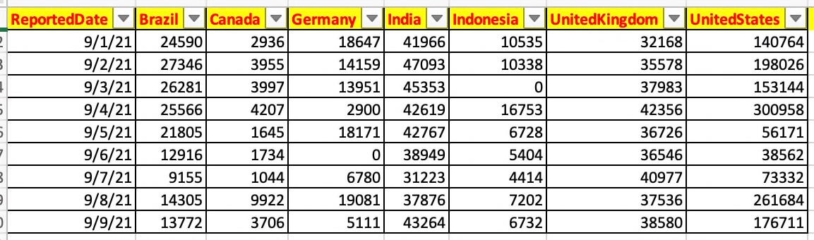
df_M.rename(columns={'ds':'ReportedDate'}, inplace=True) |
|
df_M.rename(columns={'AdjustTrend':colName}, inplace=True) |
|
|
|
return df_M |
|
except: |
|
df = p.DataFrame() |
|
|
|
return df |
|
|
|
def toPivot(inDF, colName): |
|
try: |
|
iDF = inDF |
|
|
|
iDF_Piv = iDF.pivot_table(colName, ['ReportedDate'], 'Country') |
|
iDF_Piv.reset_index( drop=False, inplace=True ) |
|
|
|
list1 = ['ReportedDate'] |
|
|
|
iDF_Arr = iDF['Country'].unique() |
|
list2 = iDF_Arr.tolist() |
|
|
|
listV = list1 + list2 |
|
|
|
iDF_Piv.reindex([listV], axis=1) |
|
|
|
return iDF_Piv |
|
except Exception as e: |
|
x = str(e) |
|
print(x) |
|
|
|
df = p.DataFrame() |
|
|
|
return df |
|
|
|
def toAgg(inDF, var, debugInd, flg): |
|
try: |
|
iDF = inDF |
|
colName = "ReportedDate" |
|
|
|
list1 = list(iDF.columns.values) |
|
list1.remove(colName) |
|
|
|
list1 = ["Brazil", "Canada", "Germany", "India", "Indonesia", "UnitedKingdom", "UnitedStates"] |
|
|
|
iDF['Year_Mon'] = iDF[colName].apply(lambda x:x.strftime('%Y%m')) |
|
iDF.drop(columns=[colName], axis=1, inplace=True) |
|
|
|
ColNameGrp = "Year_Mon" |
|
print('List1 Aggregate:: ', str(list1)) |
|
print('ColNameGrp :: ', str(ColNameGrp)) |
|
|
|
iDF_T = iDF[["Year_Mon", "Brazil", "Canada", "Germany", "India", "Indonesia", "UnitedKingdom", "UnitedStates"]] |
|
iDF_T.fillna(0, inplace = True) |
|
print('iDF_T:: ') |
|
print(iDF_T) |
|
|
|
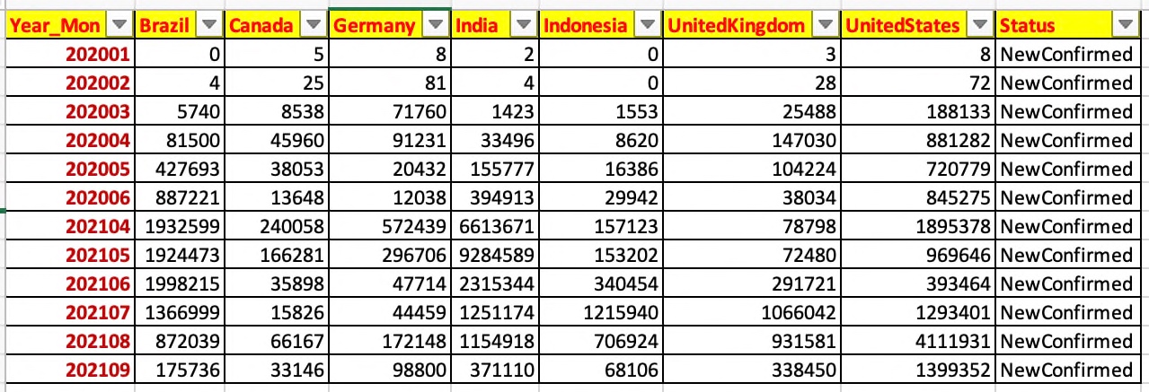
iDF_1_max_group = iDF_T.groupby(ColNameGrp, as_index=False)[list1].sum() |
|
iDF_1_max_group['Status'] = flg |
|
|
|
return iDF_1_max_group |
|
except Exception as e: |
|
x = str(e) |
|
print(x) |
|
|
|
df = p.DataFrame() |
|
|
|
return df |
|
|
|
def publishEvents(inDF1, inDF2, inDF3, inDF4, var, debugInd): |
|
try: |
|
# Original Covid Data from API |
|
iDF1 = inDF1 |
|
iDF2 = inDF2 |
|
|
|
NC = 'NewConfirmed' |
|
ND = 'NewDeaths' |
|
|
|
iDF1_PV = toPivot(iDF1, NC) |
|
iDF1_PV['ReportedDate'] = p.to_datetime(iDF1_PV['ReportedDate']) |
|
l.logr('57.iDF1_PV_' + var + '.csv', debugInd, iDF1_PV, 'log') |
|
|
|
iDF2_PV = toPivot(iDF2, ND) |
|
iDF2_PV['ReportedDate'] = p.to_datetime(iDF2_PV['ReportedDate']) |
|
l.logr('58.iDF2_PV_' + var + '.csv', debugInd, iDF2_PV, 'log') |
|
|
|
# Predicted Covid Data from Facebook API |
|
iDF3 = inDF3 |
|
iDF4 = inDF4 |
|
|
|
iDF3_PV = toPivot(iDF3, NC) |
|
l.logr('59.iDF3_PV_' + var + '.csv', debugInd, iDF3_PV, 'log') |
|
|
|
iDF4_PV = toPivot(iDF4, ND) |
|
l.logr('60.iDF4_PV_' + var + '.csv', debugInd, iDF4_PV, 'log') |
|
|
|
# Now aggregating data based on year-month only |
|
iDF1_Agg = toAgg(iDF1_PV, var, debugInd, NC) |
|
l.logr('61.iDF1_Agg_' + var + '.csv', debugInd, iDF1_Agg, 'log') |
|
|
|
iDF2_Agg = toAgg(iDF2_PV, var, debugInd, ND) |
|
l.logr('62.iDF2_Agg_' + var + '.csv', debugInd, iDF2_Agg, 'log') |
|
|
|
iDF3_Agg = toAgg(iDF3_PV, var, debugInd, NC) |
|
l.logr('63.iDF3_Agg_' + var + '.csv', debugInd, iDF3_Agg, 'log') |
|
|
|
iDF4_Agg = toAgg(iDF4_PV, var, debugInd, ND) |
|
l.logr('64.iDF4_Agg_' + var + '.csv', debugInd, iDF4_Agg, 'log') |
|
|
|
# Initiating Ably class to push events |
|
x1 = cps.clsPublishStream() |
|
|
|
# Pushing both the Historical Confirmed Cases |
|
retVal_1 = x1.pushEvents(iDF1_Agg, debugInd, var, NC) |
|
|
|
if retVal_1 == 0: |
|
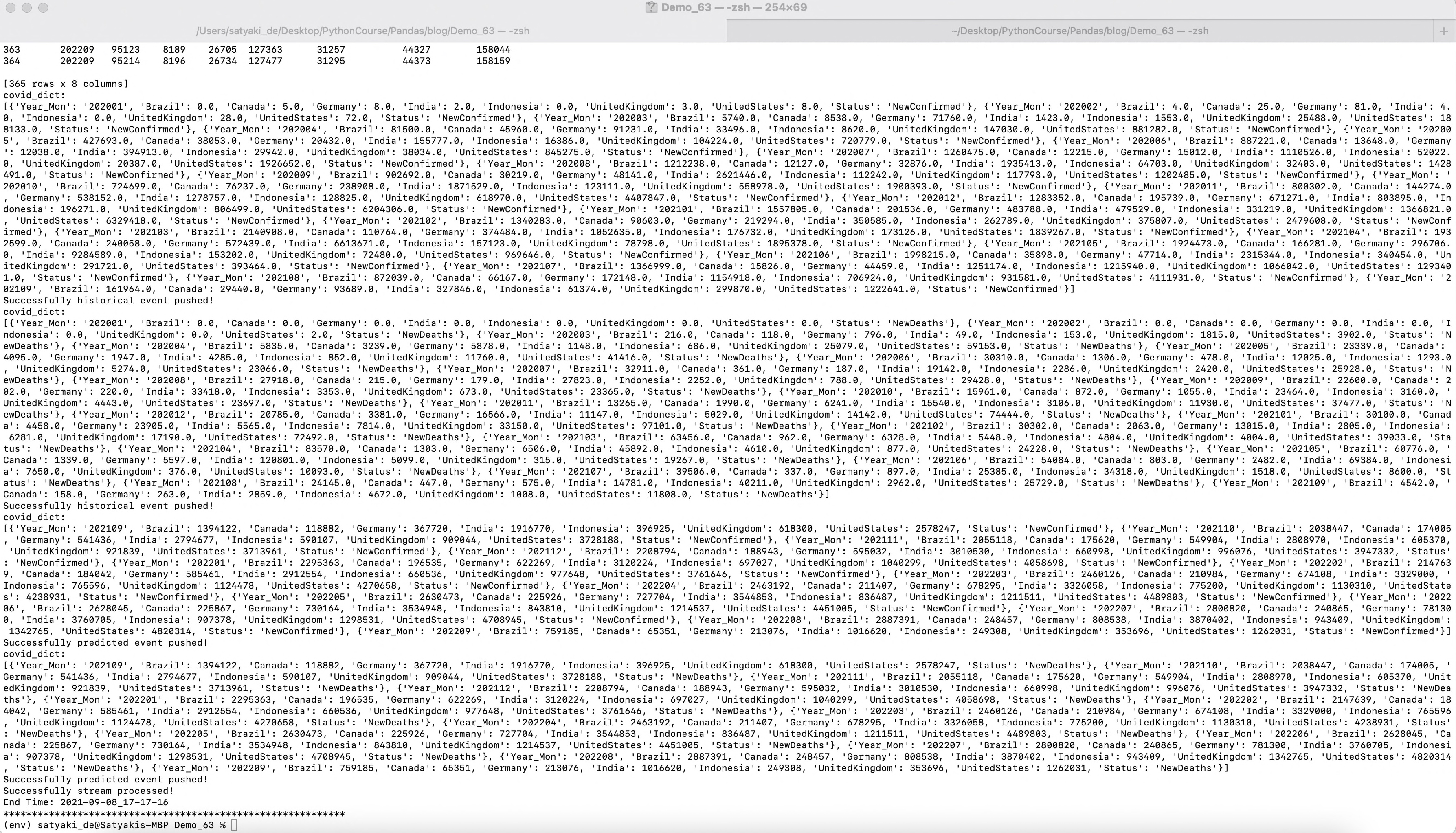
print('Successfully historical event pushed!') |
|
else: |
|
print('Failed to push historical events!') |
|
|
|
# Pushing both the Historical Death Cases |
|
retVal_3 = x1.pushEvents(iDF2_Agg, debugInd, var, ND) |
|
|
|
if retVal_3 == 0: |
|
print('Successfully historical event pushed!') |
|
else: |
|
print('Failed to push historical events!') |
|
|
|
time.sleep(5) |
|
|
|
# Pushing both the New Confirmed Cases |
|
retVal_2 = x1.pushEvents(iDF3_Agg, debugInd, var, NC) |
|
|
|
if retVal_2 == 0: |
|
print('Successfully predicted event pushed!') |
|
else: |
|
print('Failed to push predicted events!') |
|
|
|
# Pushing both the New Death Cases |
|
retVal_4 = x1.pushEvents(iDF4_Agg, debugInd, var, ND) |
|
|
|
if retVal_4 == 0: |
|
print('Successfully predicted event pushed!') |
|
else: |
|
print('Failed to push predicted events!') |
|
|
|
|
|
return 0 |
|
except Exception as e: |
|
x = str(e) |
|
|
|
print(x) |
|
|
|
return 1 |
|
|
|
def main(): |
|
try: |
|
var1 = datetime.datetime.now().strftime("%Y-%m-%d_%H-%M-%S") |
|
print('*' *60) |
|
DInd = 'Y' |
|
NC = 'New Confirmed' |
|
ND = 'New Dead' |
|
SM = 'data process Successful!' |
|
FM = 'data process Failure!' |
|
|
|
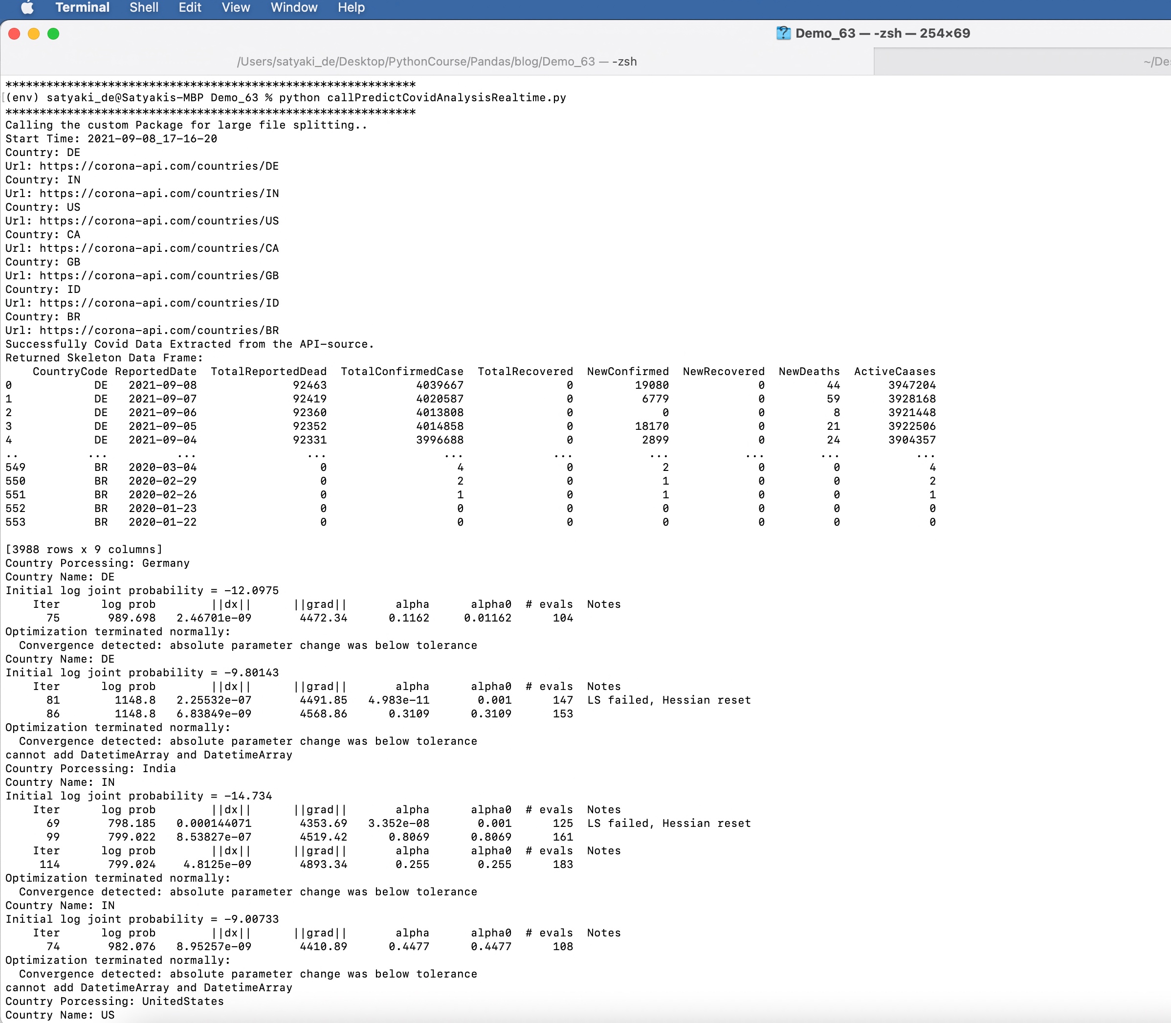
print("Calling the custom Package for large file splitting..") |
|
print('Start Time: ' + str(var1)) |
|
|
|
countryList = str(cf.conf['coList']).split(',') |
|
|
|
# Initiating Log Class |
|
general_log_path = str(cf.conf['LOG_PATH']) |
|
|
|
# Enabling Logging Info |
|
logging.basicConfig(filename=general_log_path + 'CovidAPI.log', level=logging.INFO) |
|
|
|
# Create the instance of the Covid API Class |
|
x1 = ca.clsCovidAPI() |
|
|
|
# Let's pass this to our map section |
|
retDF = x1.searchQry(var1, DInd) |
|
|
|
retVal = int(retDF.shape[0]) |
|
|
|
if retVal > 0: |
|
print('Successfully Covid Data Extracted from the API-source.') |
|
else: |
|
print('Something wrong with your API-source!') |
|
|
|
# Extracting Skeleton Data |
|
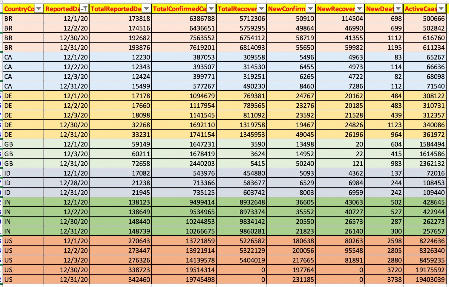
df = retDF[['data.code', 'date', 'deaths', 'confirmed', 'recovered', 'new_confirmed', 'new_recovered', 'new_deaths', 'active']] |
|
|
|
df.columns = ['CountryCode', 'ReportedDate', 'TotalReportedDead', 'TotalConfirmedCase', 'TotalRecovered', 'NewConfirmed', 'NewRecovered', 'NewDeaths', 'ActiveCaases'] |
|
|
|
df.dropna() |
|
|
|
print('Returned Skeleton Data Frame: ') |
|
print(df) |
|
|
|
l.logr('5.df_' + var1 + '.csv', DInd, df, 'log') |
|
|
|
# Due to source data issue, application will perform of |
|
# avg of counts based on dates due to multiple entries |
|
g_df = df.groupby(["CountryCode", "ReportedDate"] , as_index=False)["TotalReportedDead","TotalConfirmedCase","TotalRecovered","NewConfirmed","NewRecovered","NewDeaths","ActiveCaases"].mean() |
|
g_df['TotalReportedDead_M'] = g_df.apply(lambda row: ceilTrend(row, 'TotalReportedDead'), axis=1) |
|
g_df['TotalConfirmedCase_M'] = g_df.apply(lambda row: ceilTrend(row, 'TotalConfirmedCase'), axis=1) |
|
g_df['TotalRecovered_M'] = g_df.apply(lambda row: ceilTrend(row, 'TotalRecovered'), axis=1) |
|
g_df['NewConfirmed_M'] = g_df.apply(lambda row: ceilTrend(row, 'NewConfirmed'), axis=1) |
|
g_df['NewRecovered_M'] = g_df.apply(lambda row: ceilTrend(row, 'NewRecovered'), axis=1) |
|
g_df['NewDeaths_M'] = g_df.apply(lambda row: ceilTrend(row, 'NewDeaths'), axis=1) |
|
g_df['ActiveCaases_M'] = g_df.apply(lambda row: ceilTrend(row, 'ActiveCaases'), axis=1) |
|
|
|
# Dropping old columns |
|
g_df.drop(columns=['TotalReportedDead', 'TotalConfirmedCase', 'TotalRecovered', 'NewConfirmed', 'NewRecovered', 'NewDeaths', 'ActiveCaases'], axis=1, inplace=True) |
|
|
|
# Renaming the new columns to old columns |
|
g_df.rename(columns={'TotalReportedDead_M':'TotalReportedDead'}, inplace=True) |
|
g_df.rename(columns={'TotalConfirmedCase_M':'TotalConfirmedCase'}, inplace=True) |
|
g_df.rename(columns={'TotalRecovered_M':'TotalRecovered'}, inplace=True) |
|
g_df.rename(columns={'NewConfirmed_M':'NewConfirmed'}, inplace=True) |
|
g_df.rename(columns={'NewRecovered_M':'NewRecovered'}, inplace=True) |
|
g_df.rename(columns={'NewDeaths_M':'NewDeaths'}, inplace=True) |
|
g_df.rename(columns={'ActiveCaases_M':'ActiveCaases'}, inplace=True) |
|
|
|
l.logr('5.g_df_' + var1 + '.csv', DInd, g_df, 'log') |
|
|
|
# Working with forecast |
|
# Create the instance of the Forecast API Class |
|
x2 = f.clsForecast() |
|
|
|
# Fetching each country name & then get the details |
|
cnt = 6 |
|
cnt_x = 0 |
|
cnt_y = 0 |
|
|
|
df_M_Confirmed = p.DataFrame() |
|
df_M_Deaths = p.DataFrame() |
|
|
|
for i in countryList: |
|
try: |
|
cntryIndiv = i.strip() |
|
|
|
cntryFullName = countryDet(cntryIndiv) |
|
|
|
print('Country Porcessing: ' + str(cntryFullName)) |
|
|
|
# Creating dataframe for each country |
|
# Germany Main DataFrame |
|
dfCountry = countrySpecificDF(g_df, cntryIndiv) |
|
l.logr(str(cnt) + '.df_' + cntryIndiv + '_' + var1 + '.csv', DInd, dfCountry, 'log') |
|
|
|
# Let's pass this to our map section |
|
retDFGenNC = x2.forecastNewConfirmed(dfCountry, DInd, var1) |
|
|
|
statVal = str(NC) |
|
|
|
a1 = plot_picture(retDFGenNC, DInd, var1, cntryIndiv, statVal) |
|
|
|
# Merging with the previous Country Code data |
|
if cnt_x == 0: |
|
df_M_Confirmed = a1 |
|
else: |
|
d_frames = [df_M_Confirmed, a1] |
|
df_M_Confirmed = p.concat(d_frames) |
|
|
|
cnt_x += 1 |
|
|
|
retDFGenNC_D = x2.forecastNewDead(dfCountry, DInd, var1) |
|
|
|
statVal = str(ND) |
|
|
|
a2 = plot_picture(retDFGenNC_D, DInd, var1, cntryIndiv, statVal) |
|
|
|
# Merging with the previous Country Code data |
|
if cnt_y == 0: |
|
df_M_Deaths = a2 |
|
else: |
|
d_frames = [df_M_Deaths, a2] |
|
df_M_Deaths = p.concat(d_frames) |
|
|
|
cnt_y += 1 |
|
|
|
# Printing Proper message |
|
if (a1 + a2) == 0: |
|
oprMsg = cntryFullName + ' ' + SM |
|
print(oprMsg) |
|
else: |
|
oprMsg = cntryFullName + ' ' + FM |
|
print(oprMsg) |
|
|
|
# Resetting the dataframe value for the next iteration |
|
dfCountry = p.DataFrame() |
|
cntryIndiv = '' |
|
oprMsg = '' |
|
cntryFullName = '' |
|
a1 = 0 |
|
a2 = 0 |
|
statVal = '' |
|
|
|
cnt += 1 |
|
except Exception as e: |
|
x = str(e) |
|
print(x) |
|
|
|
l.logr('49.df_M_Confirmed_' + var1 + '.csv', DInd, df_M_Confirmed, 'log') |
|
l.logr('50.df_M_Deaths_' + var1 + '.csv', DInd, df_M_Deaths, 'log') |
|
|
|
# Removing unwanted columns |
|
df_M_Confirmed.drop(columns=['trend', 'trend_lower', 'trend_upper'], axis=1, inplace=True) |
|
df_M_Deaths.drop(columns=['trend', 'trend_lower', 'trend_upper'], axis=1, inplace=True) |
|
|
|
l.logr('51.df_M_Confirmed_' + var1 + '.csv', DInd, df_M_Confirmed, 'log') |
|
l.logr('52.df_M_Deaths_' + var1 + '.csv', DInd, df_M_Deaths, 'log') |
|
|
|
# Creating original dataframe from the source API |
|
df_M_Confirmed_Orig = g_df[['CountryCode', 'ReportedDate','NewConfirmed']] |
|
df_M_Deaths_Orig = g_df[['CountryCode', 'ReportedDate','NewDeaths']] |
|
|
|
# Transforming Country Code |
|
df_M_Confirmed_Orig['Country'] = df_M_Confirmed_Orig.apply(lambda row: lookupCountry(row), axis=1) |
|
df_M_Deaths_Orig['Country'] = df_M_Deaths_Orig.apply(lambda row: lookupCountry(row), axis=1) |
|
|
|
# Dropping unwanted column |
|
df_M_Confirmed_Orig.drop(columns=['CountryCode'], axis=1, inplace=True) |
|
df_M_Deaths_Orig.drop(columns=['CountryCode'], axis=1, inplace=True) |
|
|
|
# Reordering columns |
|
df_M_Confirmed_Orig = df_M_Confirmed_Orig.reindex(['ReportedDate','Country','NewConfirmed'], axis=1) |
|
df_M_Deaths_Orig = df_M_Deaths_Orig.reindex(['ReportedDate','Country','NewDeaths'], axis=1) |
|
|
|
l.logr('53.df_M_Confirmed_Orig_' + var1 + '.csv', DInd, df_M_Confirmed_Orig, 'log') |
|
l.logr('54.df_M_Deaths_Orig_' + var1 + '.csv', DInd, df_M_Deaths_Orig, 'log') |
|
|
|
# Filter out only the predicted data |
|
filterDF_1 = extractPredictedDF(df_M_Confirmed_Orig, df_M_Confirmed, 'NewConfirmed') |
|
l.logr('55.filterDF_1_' + var1 + '.csv', DInd, filterDF_1, 'log') |
|
|
|
filterDF_2 = extractPredictedDF(df_M_Confirmed_Orig, df_M_Confirmed, 'NewDeaths') |
|
l.logr('56.filterDF_2_' + var1 + '.csv', DInd, filterDF_2, 'log') |
|
|
|
# Calling the final publish events |
|
retVa = publishEvents(df_M_Confirmed_Orig, df_M_Deaths_Orig, filterDF_1, filterDF_2, var1, DInd) |
|
|
|
if retVa == 0: |
|
print('Successfully stream processed!') |
|
else: |
|
print('Failed to process stream!') |
|
|
|
|
|
var2 = datetime.datetime.now().strftime("%Y-%m-%d_%H-%M-%S") |
|
print('End Time: ' + str(var2)) |
|
print('*' *60) |
|
|
|
except Exception as e: |
|
x = str(e) |
|
|
|
print(x) |
|
|
|
if __name__ == "__main__": |
|
main() |


You must be logged in to post a comment.