This site mainly deals with various use cases demonstrated using Python, Data Science, Cloud basics, SQL Server, Oracle, Teradata along with SQL & their implementation. Expecting yours active participation & time. This blog can be access from your TP, Tablet & mobile also. Please provide your feedback.
This is a continuation of my previous post, which can be found here. This will be our last post of this series.
Let us recap the key takaways from our previous post –
Two cloud patterns show how MCP standardizes safe AI-to-system work. Azure “agent factory”: You ask in Teams; Azure AI Foundry dispatches a specialist agent (HR/Sales). The agent calls a specific MCP server (Functions/Logic Apps) for CRM, SharePoint, or SQL via API Management. Entra ID enforces access; Azure Monitor audits. AWS “composable serverless agents”: In Bedrock, domain agents (Financial/IT Ops) invoke Lambda-based MCP tools for DynamoDB, S3, or CloudWatch through API Gateway with IAM and optional VPC. In both, agents never hold credentials; tools map one-to-one to systems, improving security, clarity, scalability, and compliance.
In this post, we’ll discuss the GCP factory pattern.
Unified Workbench Pattern (GCP):
The GCP “unified workbench” pattern prioritizes a unified, data-centric platform for AI development, integrating seamlessly with Vertex AI and Google’s expertise in AI and data analytics. This approach is well-suited for AI-first companies and data-intensive organizations that want to build agents that leverage cutting-edge research tools.
Let’s explore the following diagram based on this –
Imagine Mia, a clinical operations lead, opens a simple app and asks: “Which clinics had the longest wait times this week? Give me a quick summary I can share.”
The app quietly sends Mia’s request to Vertex AI Agent Builder—think of it as the switchboard operator.
Vertex AI picks the Data Analysis agent (the “specialist” for questions like Mia’s).
That agent doesn’t go rummaging through databases. Instead, it uses a safe, preapproved tool—an MCP Server—to query BigQuery, where the data lives.
The tool fetches results and returns them to Mia—no passwords in the open, no risky shortcuts—just the answer, fast and safely.
Now meet Ravi, a developer who asks: “Show me the latest app metrics and confirm yesterday’s patch didn’t break the login table.”
The app routes Ravi’s request to Vertex AI.
Vertex AI chooses the Developer agent.
That agent calls a different tool—an MCP Server designed for Cloud SQL—to check the login table and run a safe query.
Results come back with guardrails intact. If the agent ever needs files, there’s also a Cloud Storage tool ready to fetch or store documents.
Let us understand how the underlying flow of activities took place –
User Interface:
Entry point: Vertex AI console or a custom app.
Sends a single request; no direct credentials or system access exposed to the user.
Orchestration: Vertex AI Agent Builder (MCP Host)
Routes the request to the most suitable agent:
Agent A (Data Analysis) for analytics/BI-style questions.
Agent B (Developer) for application/data-ops tasks.
Tooling via MCP Servers on Cloud Run
Each MCP Server is a purpose-built adapter with least-privilege access to exactly one service:
Server1 → BigQuery (analytics/warehouse) — used by Agent A in this diagram.
Server2 → Cloud Storage (GCS) (files/objects) — available when file I/O is needed.
Server3 → Cloud SQL (relational DB) — used by Agent B in this diagram.
Agents never hold database credentials; they request actions from the right tool.
Enterprise Systems
BigQuery, Cloud Storage, and Cloud SQL are the systems of record that the tools interact with.
Security, Networking, and Observability
GCP IAM: AuthN/AuthZ for Vertex AI and each MCP Server (fine-grained roles, least privilege).
GCP VPC: Private network paths for all Cloud Run MCP Servers (isolation, egress control).
Cloud Monitoring: Metrics, logs, and alerts across agents and tools (auditability, SLOs).
Return Path
Results flow back from the service → MCP Server → Agent → Vertex AI → UI.
Policies and logs track who requested what, when, and how.
Why does this design work?
One entry point for questions.
Clear accountability: specialists (agents) act within guardrails.
Built-in safety (IAM/VPC) and visibility (Monitoring) for trust.
Separation of concerns: agents decide what to do; tools (MCP Servers) decide how to do it.
Scalable: add a new tool (e.g., Pub/Sub or Vertex AI Feature Store) without changing the UI or agents.
Auditable & maintainable: each tool maps to one service with explicit IAM and VPC controls.
So, we’ve concluded the series with the above post. I hope you like it.
I’ll bring some more exciting topics in the coming days from the new advanced world of technology.
Till then, Happy Avenging! 🙂
Note: All the data & scenarios posted here are representative of data & scenarios available on the internet for educational purposes only. There is always room for improvement in this kind of model & the solution associated with it. I’ve shown the basic ways to achieve the same for educational purposes only.
This is a continuation of my previous post, which can be found here.
Let us recap the key takaways from our previous post –
The Model Context Protocol (MCP) standardizes how AI agents use tools and data. Instead of fragile, custom connectors (N×M problem), teams build one MCP server per system; any MCP-compatible agent can use it, reducing cost and breakage. Unlike RAG, which retrieves static, unstructured documents for context, MCP enables live, structured, and actionable operations (e.g., query databases, create tickets). Compared with proprietary plugins, MCP is open, model-agnostic (JSON-RPC 2.0), and minimizes vendor lock-in. Cloud patterns: Azure “agent factory,” AWS “serverless agents,” and GCP “unified workbench”—each hosting agents with MCP servers securely fronting enterprise services.
Today, we’ll try to understand some of the popular pattern from the world of cloud & we’ll explore them in this post & the next post.
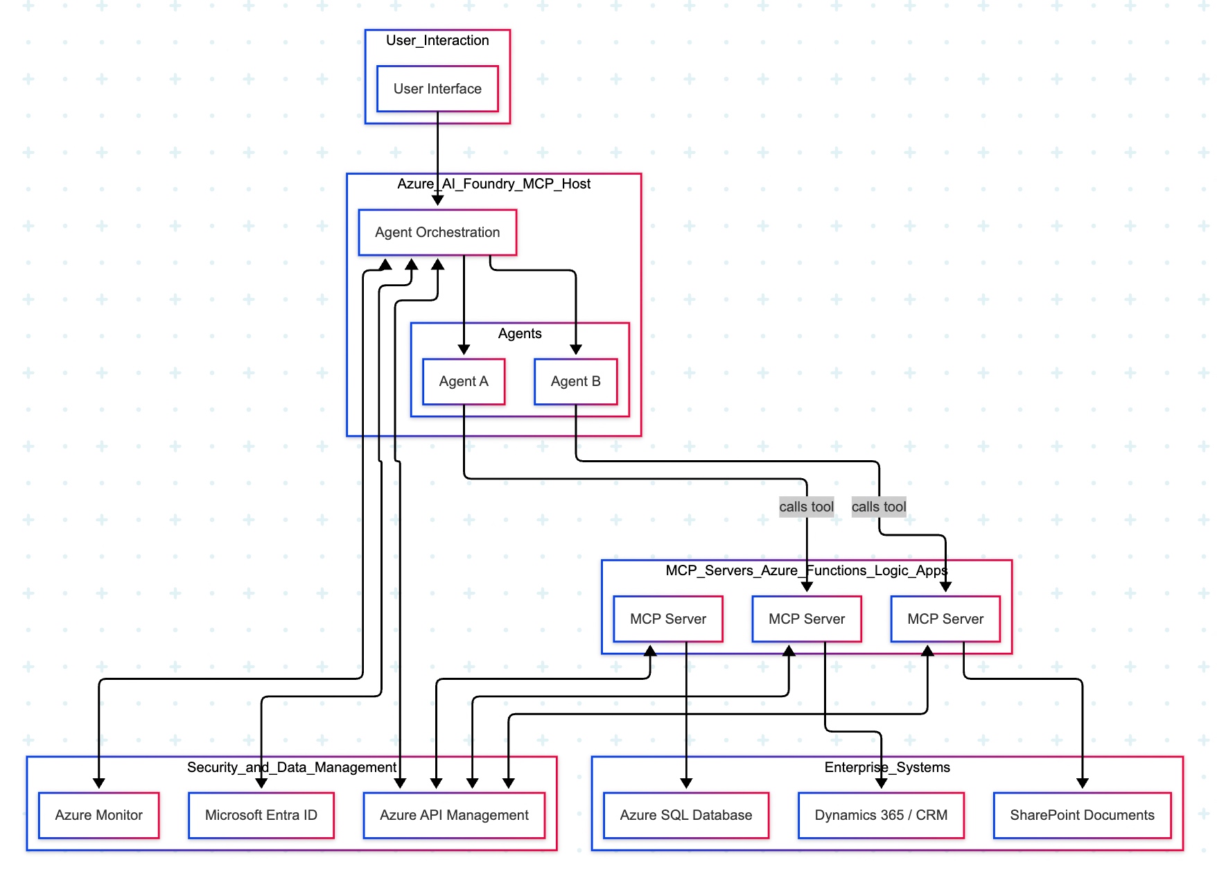
Agent Factory Pattern (Azure):
The Azure “agent factory” pattern leverages the Azure AI Foundry to serve as a secure, managed hub for creating and orchestrating multiple specialized AI agents. This pattern emphasizes enterprise-grade security, governance, and seamless integration with the Microsoft ecosystem, making it ideal for organizations that use Microsoft products extensively.
Let’s explore the following diagram based on this –
Imagine you ask a question in Microsoft Teams—“Show me the latest HR policy” or “What is our current sales pipeline?” Your message is sent to Azure AI Foundry, which acts as an expert dispatcher. Foundry chooses a specialist AI agent—for example, an HR agent for policies or a Sales agent for the pipeline.
That agent does not rummage through your systems directly. Instead, it uses a safe, preapproved tool (an “MCP Server”) that knows how to talk to one system—such as Dynamics 365/CRM, SharePoint, or an Azure SQL database. The tool gets the information, sends it back to the agent, who then explains the answer clearly to you in Teams.
Throughout the process, three guardrails keep everything safe and reliable:
Microsoft Entra ID checks identity and permissions.
Azure API Management (APIM) is the controlled front door for all tool calls.
Azure Monitor watches performance and creates an audit trail.
Let us now understand the technical events that is going on underlying this request –
Control plane: Azure AI Foundry (MCP Host) orchestrates intent, tool selection, and multi-agent flows.
Execution plane: Agents invoke MCP Servers (Azure Functions/Logic Apps) via APIM; each server encapsulates a single domain integration (CRM, SharePoint, SQL).
Data plane:
MCP Server (CRM) ↔ Dynamics 365/CRM
MCP Server (SharePoint) ↔ SharePoint
MCP Server (SQL) ↔ Azure SQL Database
Identity & access:Entra ID issues tokens and enforces least-privilege access; Foundry, APIM, and MCP Servers validate tokens.
Observability:Azure Monitor for metrics, logs, distributed traces, and auditability across agents and tool calls.
Traffic pattern in diagram:
User → Foundry → Agent (Sales/HR).
Agent —tool call→ MCP Server (CRM/SharePoint/SQL).
MCP Server → Target system; response returns along the same path.
Note: The SQL MCP Server is shown connected to Azure SQL; agents can call it in the same fashion as CRM/SharePoint when a use case requires relational data.
Why does this design work?
Safety by design: Agents never directly touch back-end systems; MCP Servers mediate access with APIM and Entra ID.
Clarity & maintainability: Each tool maps to one system; changes are localized and testable.
Scalability: Add new agents or systems by introducing another MCP Server behind APIM.
Auditability: Every action is observable in Azure Monitor for compliance and troubleshooting.
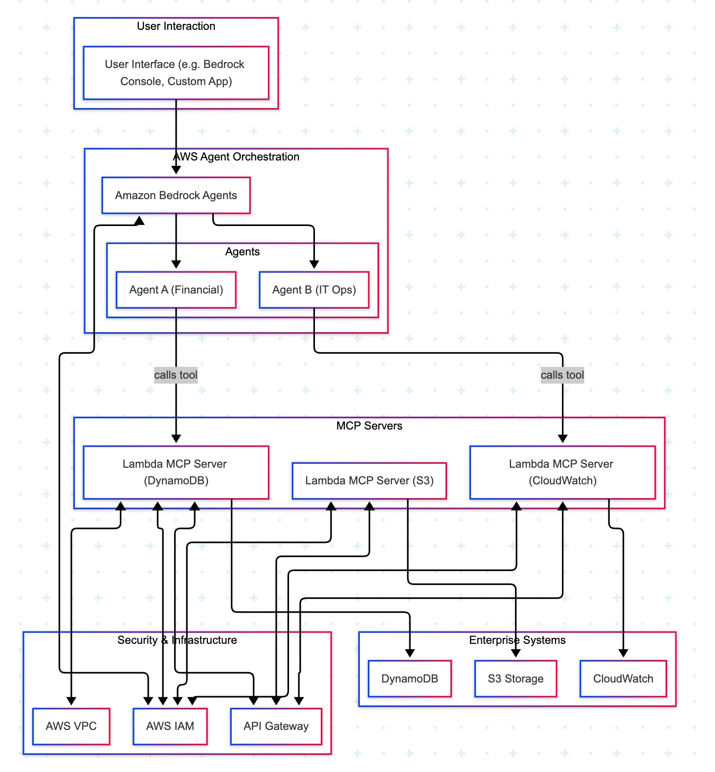
AWS MCP Architecture:
The AWS “composable serverless agent” pattern focuses on building lightweight, modular, and event-driven AI agents using Bedrock and serverless technologies. It prioritizes customization, scalability, and leveraging AWS’s deep service portfolio, making it a strong choice for enterprises that value flexibility and granular control.
A manager opens a familiar app (the Bedrock console or a simple web app) and types, “Show me last quarter’s approved purchase requests.” The request goes to Amazon Bedrock Agents, which acts like an intelligent dispatcher. It chooses the Financial Agent—a specialist in finance tasks. That agent uses a safe, pre-approved tool to fetch data from the company’s DynamoDB records. Moments later, the manager sees a clear summary, without ever touching databases or credentials.
Actors & guardrails. UI (Bedrock console or custom app) → Amazon Bedrock Agents (MCP host/orchestrator) → Domain Agents (Financial, IT Ops) → MCP Servers on AWS Lambda (one tool per AWS service) → Enterprise Services (DynamoDB, S3, CloudWatch). Access is governed by IAM (least-privilege roles, agent→tool→service), ingress/policy by API Gateway (front door to each Lambda tool), and network isolation by VPC where required.
Agent–tool mappings:
Agent A (Financial) → Lambda MCP (DynamoDB)
Agent B (IT Ops) → Lambda MCP (CloudWatch)
Optional: Lambda MCP (S3) for file/object operations
End-to-end sequence:
UI → Bedrock Agents: User submits a prompt.
Agent selection: Bedrock dispatches to the appropriate domain agent (Financial or IT Ops).
Tool invocation: The agent calls the required Lambda MCP Server via API Gateway.
Authorization: The tool executes only permitted actions under its IAM role (least privilege).
Safer by default: Agents never handle raw credentials; tools enforce least privilege with IAM.
Clear boundaries: Each tool maps to one service, making audits and changes simpler.
Scalable & maintainable:Lambda and API Gateway scale on demand; adding a new tool (e.g., a Cost Explorer tool) does not require changing the UI or existing agents.
Faster delivery: Specialists (agents) focus on logic; tools handle system specifics.
In the next post, we’ll conclude the final thread on this topic.
Till then, Happy Avenging! 🙂
Note: All the data & scenarios posted here are representational data & scenarios & available over the internet & for educational purposes only. There is always room for improvement in this kind of model & the solution associated with it. I’ve shown the basic ways to achieve the same for educational purposes only.
This is a continuation of my previous post, which can be found here.
Let us recap the key takaways from our previous post –
Enterprise AI, utilizing the Model Context Protocol (MCP), leverages an open standard that enables AI systems to securely and consistently access enterprise data and tools. MCP replaces brittle “N×M” integrations between models and systems with a standardized client–server pattern: an MCP host (e.g., IDE or chatbot) runs an MCP client that communicates with lightweight MCP servers, which wrap external systems via JSON-RPC. Servers expose three assets—Resources (data), Tools (actions), and Prompts (templates)—behind permissions, access control, and auditability. This design enables real-time context, reduces hallucinations, supports model- and cloud-agnostic interoperability, and accelerates “build once, integrate everywhere” deployment. A typical flow (e.g., retrieving a customer’s latest order) encompasses intent parsing, authorized tool invocation, query translation/execution, and the return of a normalized JSON result to the model for natural-language delivery. Performance introduces modest overhead (RPC hops, JSON (de)serialization, network transit) and scale considerations (request volume, significant results, context-window pressure). Mitigations include in-memory/semantic caching, optimized SQL with indexing, pagination, and filtering, connection pooling, and horizontal scaling with load balancing. In practice, small latency costs are often outweighed by the benefits of higher accuracy, stronger governance, and a decoupled, scalable architecture.
How does MCP compare with other AI integration approaches?
Compared to other approaches, the Model Context Protocol (MCP) offers a uniquely standardized and secure framework for AI-tool integration, shifting from brittle, custom-coded connections to a universal plug-and-play model. It is not a replacement for underlying systems, such as APIs or databases, but instead acts as an intelligent, secure abstraction layer designed explicitly for AI agents.
MCP vs. Custom API integrations:
This approach was the traditional method for AI integration before standards like MCP emerged.
Custom API integrations (traditional): Each AI application requires a custom-built connector for every external system it needs to access, leading to an N x M integration problem (the number of connectors grows exponentially with the number of models and systems). This approach is resource-intensive, challenging to maintain, and prone to breaking when underlying APIs change.
MCP: The standardized protocol eliminates the N x M problem by creating a universal interface. Tool creators build a single MCP server for their system, and any MCP-compatible AI agent can instantly access it. This process decouples the AI model from the underlying implementation details, drastically reducing integration and maintenance costs.
For more detailed information, please refer to the following link.
MCP vs. Retrieval-Augmented Generation (RAG):
RAG is a technique that retrieves static documents to augment an LLM’s knowledge, while MCP focuses on live interactions. They are complementary, not competing.
RAG:
Focus: Retrieving and summarizing static, unstructured data, such as documents, manuals, or knowledge bases.
Best for: Providing background knowledge and general information, as in a policy lookup tool or customer service bot.
Data type: Unstructured, static knowledge.
MCP:
Focus: Accessing and acting on real-time, structured, and dynamic data from databases, APIs, and business systems.
Best for: Agentic use cases involving real-world actions, like pulling live sales reports from a CRM or creating a ticket in a project management tool.
Data type: Structured, real-time, and dynamic data.
MCP vs. LLM plugins and extensions:
Before MCP, platforms like OpenAI offered proprietary plugin systems to extend LLM capabilities.
LLM plugins:
Proprietary: Tied to a specific AI vendor (e.g., OpenAI).
Limited: Rely on the vendor’s API function-calling mechanism, which focuses on call formatting but not standardized execution.
Centralized: Managed by the AI vendor, creating a risk of vendor lock-in.
MCP:
Open standard: Based on a public, interoperable protocol (JSON-RPC 2.0), making it model-agnostic and usable across different platforms.
Infrastructure layer: Provides a standardized infrastructure for agents to discover and use any compliant tool, regardless of the underlying LLM.
Decentralized: Promotes a flexible ecosystem and reduces the risk of vendor lock-in.
How enterprise AI with MCP has opened up a specific Architecture pattern for Azure, AWS & GCP?
Microsoft Azure:
The “agent factory” pattern: Azure focuses on providing managed services for building and orchestrating AI agents, tightly integrated with its enterprise security and governance features. The MCP architecture is a core component of the Azure AI Foundry, serving as a secure, managed “agent factory.”
Azure architecture pattern with MCP:
AI orchestration layer: The Azure AI Agent Service, within Azure AI Foundry, acts as the central host and orchestrator. It provides the control plane for creating, deploying, and managing multiple specialized agents, and it natively supports the MCP standard.
AI model layer: Agents in the Foundry can be powered by various models, including those from Azure OpenAI Service, commercial models from partners, or open-source models.
MCP server and tool layer: MCP servers are deployed using serverless functions, such as Azure Functions or Azure Logic Apps, to wrap existing enterprise systems. These servers expose tools for interacting with enterprise data sources like SharePoint, Azure AI Search, and Azure Blob Storage.
Data and security layer: Data is secured using Microsoft Entra ID (formerly Azure AD) for authentication and access control, with robust security policies enforced via Azure API Management. Access to data sources, such as databases and storage, is managed securely through private networks and Managed Identity.
Amazon Web Services (AWS):
The “composable serverless agent” pattern: AWS emphasizes a modular, composable, and serverless approach, leveraging its extensive portfolio of services to build sophisticated, flexible, and scalable AI solutions. The MCP architecture here aligns with the principle of creating lightweight, event-driven services that AI agents can orchestrate.
AWS architecture pattern with MCP:
The AI orchestration layer, which includesAmazon Bedrock Agents or custom agent frameworks deployed via AWS Fargate or Lambda, acts as the MCP hosts. Bedrock Agents provide built-in orchestration, while custom agents offer greater flexibility and customization options.
AI model layer: The models are sourced from Amazon Bedrock, which provides a wide selection of foundation models.
MCP server and tool layer: MCP servers are deployed as serverless AWS Lambda functions. AWS offers pre-built MCP servers for many of its services, including the AWS Serverless MCP Server for managing serverless applications and the AWS Lambda Tool MCP Server for invoking existing Lambda functions as tools.
Data and security layer: Access is tightly controlled using AWS Identity and Access Management (IAM) roles and policies, with fine-grained permissions for each MCP server. Private data sources like databases (Amazon DynamoDB) and storage (Amazon S3) are accessed securely within a Virtual Private Cloud (VPC).
Google Cloud Platform (GCP):
The “unified workbench” pattern: GCP focuses on providing a unified, open, and data-centric platform for AI development. The MCP architecture on GCP integrates natively with the Vertex AI platform, treating MCP servers as first-class tools that can be dynamically discovered and used within a single workbench.
GCP architecture pattern with MCP:
AI orchestration layer: The Vertex AI Agent Builder serves as the central environment for building and managing conversational AI and other agents. It orchestrates workflows and manages tool invocation for agents.
AI model layer: Agents use foundation models available through the Vertex AI Model Garden or the Gemini API.
MCP server and tool layer: MCP servers are deployed as containerized microservices on Cloud Run or managed by services like App Engine. These servers contain tools that interact with GCP services, such as BigQuery, Cloud Storage, and Cloud SQL. GCP offers pre-built MCP server implementations, such as the GCP MCP Toolbox, for integration with its databases.
Data and security layer:Vertex AI Vector Search and other data sources are encapsulated within the MCP server tools to provide contextual information. Access to these services is managed by Identity and Access Management (IAM) and secured through virtual private clouds. The MCP server can leverage Vertex AI Context Caching for improved performance.
Note that all the native technology is referred to in each respective cloud. Hence, some of the better technologies can be used in place of the tool mentioned here. This is more of a concept-level comparison rather than industry-wise implementation approaches.
We’ll go ahead and conclude this post here & continue discussing on a further deep dive in the next post.
Till then, Happy Avenging! 🙂
Note: All the data & scenarios posted here are representational data & scenarios & available over the internet & for educational purposes only. There is always room for improvement in this kind of model & the solution associated with it. I’ve shown the basic ways to achieve the same for educational purposes only.
This is a continuation of my previous post, which can be found here.
Let us recap the key takaways from our previous post –
Agentic AI refers to autonomous systems that pursue goals with minimal supervision by planning, reasoning about next steps, utilizing tools, and maintaining context across sessions. Core capabilities include goal-directed autonomy, interaction with tools and environments (e.g., APIs, databases, devices), multi-step planning and reasoning under uncertainty, persistence, and choiceful decision-making.
Architecturally, three modules coordinate intelligent behavior: Sensing (perception pipelines that acquire multimodal data, extract salient patterns, and recognize entities/events); Observation/Deliberation (objective setting, strategy formation, and option evaluation relative to resources and constraints); and Action (execution via software interfaces, communications, or physical actuation to deliver outcomes). These functions are enabled by machine learning, deep learning, computer vision, natural language processing, planning/decision-making, uncertainty reasoning, and simulation/modeling.
At enterprise scale, open standards align autonomy with governance: the Model Context Protocol (MCP) grants an agent secure, principled access to enterprise tools and data (vertical integration), while Agent-to-Agent (A2A) enables specialized agents to coordinate, delegate, and exchange information (horizontal collaboration). Together, MCP and A2A help organizations transition from isolated pilots to scalable programs, delivering end-to-end automation, faster integration, enhanced security and auditability, vendor-neutral interoperability, and adaptive problem-solving that responds to real-time context.
Great! Let’s dive into this topic now.
Enterprise AI with MCP refers to the application of the Model Context Protocol (MCP), an open standard, to enable AI systems to securely and consistently access external enterprise data and applications.
The problem MCP solves in enterprise AI:
Before MCP, enterprise AI integration was characterized by a “many-to-many” or “N x M” problem. Companies had to build custom, fragile, and costly integrations between each AI model and every proprietary data source, which was not scalable. These limitations left AI agents with limited, outdated, or siloed information, restricting their potential impact. MCP addresses this by offering a standardized architecture for AI and data systems to communicate with each other.
How does MCP work?
The MCP framework uses a client-server architecture to enable communication between AI models and external tools and data sources.
MCP Host: The AI-powered application or environment, such as an AI-enhanced IDE or a generative AI chatbot like Anthropic’s Claude or OpenAI’s ChatGPT, where the user interacts.
MCP Client: A component within the host application that manages the connection to MCP servers.
MCP Server: A lightweight service that wraps around an external system (e.g., a CRM, database, or API) and exposes its capabilities to the AI client in a standardized format, typically using JSON-RPC 2.0.
An MCP server provides AI clients with three key resources:
Resources: Structured or unstructured data that an AI can access, such as files, documents, or database records.
Tools: The functionality to perform specific actions within an external system, like running a database query or sending an email.
Prompts: Pre-defined text templates or workflows to help guide the AI’s actions.
Benefits of MCP for enterprise AI:
Standardized integration: Developers can build integrations against a single, open standard, which dramatically reduces the complexity and time required to deploy and scale AI initiatives.
Enhanced security and governance: MCP incorporates native support for security and compliance measures. It provides permission models, access control, and auditing capabilities to ensure AI systems only access data and tools within specified boundaries.
Real-time contextual awareness: By connecting AI agents to live enterprise data sources, MCP ensures they have access to the most current and relevant information, which reduces hallucinations and improves the accuracy of AI outputs.
Greater interoperability: MCP is model-agnostic & can be used with a variety of AI models (e.g., Anthropic’s Claude or OpenAI’s models) and across different cloud environments. This approach helps enterprises avoid vendor lock-in.
Accelerated development: The “build once, integrate everywhere” approach enables internal teams to focus on innovation instead of writing custom connectors for every system.
Flow of activities:
Let us understand one sample case & the flow of activities.
A customer support agent uses an AI assistant to get information about a customer’s recent orders. The AI assistant utilizes an MCP-compliant client to communicate with an MCP server, which is connected to the company’s PostgreSQL database.
The interaction flow:
1. User request: The support agent asks the AI assistant, “What was the most recent order placed by Priyanka Chopra Jonas?”
2. AI model processes intent: The AI assistant, running on an MCP host, analyzes the natural language query. It recognizes that to answer this question, it needs to perform a database query. It then identifies the appropriate tool from the MCP server’s capabilities.
3. Client initiates tool call: The AI assistant’s MCP client sends a JSON-RPC request to the MCP server connected to the PostgreSQL database. The request specifies the tool to be used, such as get_customer_orders, and includes the necessary parameters:
5. Database returns data: The PostgreSQL database executes the query and returns the requested data to the MCP server.
6. Server formats the response: The MCP server receives the raw database output and formats it into a standardized JSON response that the MCP client can understand.
7. Client returns data to the model: The MCP client receives the JSON response and passes it back to the AI assistant’s language model.
8. AI model generates final response: The language model incorporates this real-time data into its response and presents it to the user in a natural, conversational format.
“Priyanka Chopra Jonas’s most recent order was placed on August 25, 2025, with an order ID of 98765, for a total of $11025.50.”
What are the performance implications of using MCP for database access?
Using the Model Context Protocol (MCP) for database access introduces a layer of abstraction that affects performance in several ways. While it adds some latency and processing overhead, strategic implementation can mitigate these effects. For AI applications, the benefits often outweigh the costs, particularly in terms of improved accuracy, security, and scalability.
Sources of performance implications::
Added latency and processing overhead:
The MCP architecture introduces extra communication steps between the AI agent and the database, each adding a small amount of latency.
RPC overhead: The JSON-RPC call from the AI’s client to the MCP server adds a small processing and network delay. This is an out-of-process request, as opposed to a simple local function call.
JSON serialization: Request and response data must be serialized and deserialized into JSON format, which requires processing time.
Network transit: For remote MCP servers, the data must travel over the network, adding latency. However, for a local or on-premise setup, this is minimal. The physical location of the MCP server relative to the AI model and the database is a significant factor.
Scalability and resource consumption:
The performance impact scales with the complexity and volume of the AI agent’s interactions.
High request volume: A single AI agent working on a complex task might issue dozens of parallel database queries. In high-traffic scenarios, managing numerous simultaneous connections can strain system resources and require robust infrastructure.
Excessive data retrieval: A significant performance risk is an AI agent retrieving a massive dataset in a single query. This process can consume a large number of tokens, fill the AI’s context window, and cause bottlenecks at the database and client levels.
Context window usage: Tool definitions and the results of tool calls consume space in the AI’s context window. If a large number of tools are in use, this can limit the AI’s “working memory,” resulting in slower and less effective reasoning.
Optimizations for high performance::
Caching:
Caching is a crucial strategy for mitigating the performance overhead of MCP.
In-memory caching: The MCP server can cache results from frequent or expensive database queries in memory (e.g., using Redis or Memcached). This approach enables repeat requests to be served almost instantly without requiring a database hit.
Semantic caching: Advanced techniques can cache the results of previous queries and serve them for semantically similar future requests, reducing token consumption and improving speed for conversational applications.
Efficient queries and resource management:
Designing the MCP server and its database interactions for efficiency is critical.
Optimized SQL: The MCP server should generate optimized SQL queries. Database indexes should be utilized effectively to expedite lookups and minimize load.
Pagination and filtering: To prevent a single query from overwhelming the system, the MCP server should implement pagination. The AI agent can be prompted to use filtering parameters to retrieve only the necessary data.
Connection pooling: This technique reuses existing database connections instead of opening a new one for each request, thereby reducing latency and database load.
Load balancing and scaling:
For large-scale enterprise deployments, scaling is essential for maintaining performance.
Multiple servers: The workload can be distributed across various MCP servers. One server could handle read requests, and another could handle writes.
Load balancing: A reverse proxy or other load-balancing solution can distribute incoming traffic across MCP server instances. Autoscaling can dynamically add or remove servers in response to demand.
The performance trade-off in perspective:
For AI-driven tasks, a slight increase in latency for database access is often a worthwhile trade-off for significant gains.
Improved accuracy: Accessing real-time, high-quality data through MCP leads to more accurate and relevant AI responses, reducing “hallucinations”.
Scalable ecosystem: The standardization of MCP reduces development overhead and allows for a more modular, scalable ecosystem, which saves significant engineering resources compared to building custom integrations.
Decoupled architecture: The MCP server decouples the AI model from the database, allowing each to be optimized and scaled independently.
We’ll go ahead and conclude this post here & continue discussing on a further deep dive in the next post.
Till then, Happy Avenging! 🙂
Note: All the data & scenarios posted here are representational data & scenarios & available over the internet & for educational purposes only. There is always room for improvement in this kind of model & the solution associated with it. I’ve shown the basic ways to achieve the same for educational purposes only.
Today, we won’t be discussing any solutions. Today, we’ll be discussing the Agentic AI & its implementation in the Enterprise landscape in a series of upcoming posts.
So, hang tight! We’re about to launch a new venture as part of our knowledge drive.
What is Agentic AI?
Agentic AI refers to artificial intelligence systems that can act autonomously to achieve goals, making decisions and taking actions without constant human oversight. Unlike traditional AI, which responds to prompts, agentic AI can plan, reason about next steps, utilize tools, and work toward objectives over extended periods of time.
Key characteristics of agentic AI include:
Autonomy and Goal-Directed Behavior: These systems can pursue objectives independently, breaking down complex tasks into smaller steps and executing them sequentially.
Tool Use and Environment Interaction: Agentic AI can interact with external systems, APIs, databases, and software tools to gather information and perform actions in the real world.
Planning and Reasoning: They can develop multi-step strategies, adapt their approach based on feedback, and reason through problems to find solutions.
Persistence: Unlike single-interaction AI, agentic systems can maintain context and continue working on tasks across multiple interactions or sessions.
Decision Making: They can evaluate options, weigh trade-offs, and make choices about how to proceed when faced with uncertainty.
Foundational Elements of Agentic AI Architectures:
Agentic AI systems have several interconnected components that work together to enable intelligent behaviour. Each element plays a crucial role in the overall functioning of the AI system, and they must interact seamlessly to achieve desired outcomes. Let’s explore each of these components in more detail.
Sensing:
The sensing module serves as the AI’s eyes and ears, enabling it to understand its surroundings and make informed decisions. Think of it as the system that helps the AI “see” and “hear” the world around it, much like how humans use their senses.
Gathering Information: The system collects data from multiple sources, including cameras for visual information, microphones for audio, sensors for physical touch, and digital systems for data. This step provides the AI with a comprehensive understanding of what’s happening.
Making Sense of Data: Raw information from sensors can be messy and overwhelming. This component processes the data to identify the essential patterns and details that actually matter for making informed decisions.
Recognizing What’s Important: Utilizing advanced techniques such as computer vision (for images), natural language processing (for text and speech), and machine learning (for data patterns), the system identifies and understands objects, people, events, and situations within the environment.
This sensing capability enables AI systems to transition from merely following pre-programmed instructions to genuinely understanding their environment and making informed decisions based on real-world conditions. It’s the difference between a basic automated system and an intelligent agent that can adapt to changing situations.
Observation:
The observation module serves as the AI’s decision-making center, where it sets objectives, develops strategies, and selects the most effective actions to take. This step is where the AI transforms what it perceives into purposeful action, much like humans think through problems and devise plans.
Setting Clear Objectives: The system establishes specific goals and desired outcomes, giving the AI a clear sense of direction and purpose. This approach helps ensure all actions are working toward meaningful results rather than random activity.
Strategic Planning: Using information about its own capabilities and the current situation, the AI creates step-by-step plans to reach its goals. It considers potential obstacles, available resources, and different approaches to find the most effective path forward.
Intelligent Decision-Making: When faced with multiple options, the system evaluates each choice against the current circumstances, established goals, and potential outcomes. It then selects the action most likely to move the AI closer to achieving its objectives.
This observation capability is what transforms an AI from a simple tool that follows commands into an intelligent system that can work independently toward business goals. It enables the AI to handle complex, multi-step tasks and adapt its approach when conditions change, making it valuable for a wide range of applications, from customer service to project management.
Action:
The action module serves as the AI’s hands and voice, turning decisions into real-world results. This step is where the AI actually puts its thinking and planning into action, carrying out tasks that make a tangible difference in the environment.
Control Systems: The system utilizes various tools to interact with the world, including motors for physical movement, speakers for communication, network connections for digital tasks, and software interfaces for system operation. These serve as the AI’s means of reaching out and making adjustments.
Task Implementation: Once the cognitive module determines the action to take, this component executes the actual task. Whether it’s sending an email, moving a robotic arm, updating a database, or scheduling a meeting, this module handles the execution from start to finish.
This action capability is what makes AI systems truly useful in business environments. Without it, an AI could analyze data and make significant decisions, but it couldn’t help solve problems or complete tasks. The action module bridges the gap between artificial intelligence and real-world impact, enabling AI to automate processes, respond to customers, manage systems, and deliver measurable business value.
Technology that is primarily involved in the Agentic AI is as follows –
1. Machine Learning
2. Deep Learning
3. Computer Vision
4. Natural Language Processing (NLP)
5. Planning and Decision-Making
6. Uncertainty and Reasoning
7. Simulation and Modeling
Agentic AI at Scale: MCP + A2A:
In an enterprise setting, agentic AI systems utilize the Model Context Protocol (MCP) and the Agent-to-Agent (A2A) protocol as complementary, open standards to achieve autonomous, coordinated, and secure workflows. An MCP-enabled agent gains the ability to access and manipulate enterprise tools and data. At the same time, A2A allows a network of these agents to collaborate on complex tasks by delegating and exchanging information.
This combined approach allows enterprises to move from isolated AI experiments to strategic, scalable, and secure AI programs.
How do the protocols work together in an enterprise?
Protocol
Function in Agentic AI
Focus
Example use case
Model Context Protocol (MCP)
Equips a single AI agent with the tools and data it needs to perform a specific job.
Vertical integration: connecting agents to enterprise systems like databases, CRMs, and APIs.
A sales agent uses MCP to query the company CRM for a client’s recent purchase history.
Agent-to-Agent (A2A)
Enables multiple specialized agents to communicate, delegate tasks, and collaborate on a larger, multi-step goal.
Horizontal collaboration: allowing agents from different domains to work together seamlessly.
An orchestrating agent uses A2A to delegate parts of a complex workflow to specialized HR, IT, and sales agents.
Advantages for the enterprise:
End-to-end automation: Agents can handle tasks from start to finish, including complex, multi-step workflows, autonomously.
Greater agility and speed: Enterprise-wide adoption of these protocols reduces the cost and complexity of integrating AI, accelerating deployment timelines for new applications.
Enhanced security and governance: Enterprise AI platforms built on these open standards incorporate robust security policies, centralized access controls, and comprehensive audit trails.
Vendor neutrality and interoperability: As open standards, MCP and A2A allow AI agents to work together seamlessly, regardless of the underlying vendor or platform.
Adaptive problem-solving: Agents can dynamically adjust their strategies and collaborate based on real-time data and contextual changes, leading to more resilient and efficient systems.
We will discuss this topic further in our upcoming posts.
Till then, Happy Avenging! 🙂
Note: All the data & scenarios posted here are representational data & scenarios & available over the internet & for educational purposes only. There is always room for improvement in this kind of model & the solution associated with it. I’ve shown the basic ways to achieve the same for educational purposes only.
Today, I’ll share one of the important posts on predicting data using facebook’s relatively new machine-learning-based API. I find this API is interesting as to how it can build & anticipate the outcome.
We’ll be using one of the most acceptable API-based sources for Covid-19 & I’ll be sharing the link over here.
We’ll be using the prophet-API developed by Facebook to predict the data. You will get the details from this link.
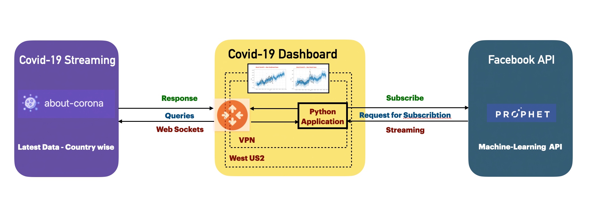
Architecture
Now, let’s explore the architecture shared above.
As you can see that the application will consume the data from the third-party API named “about-corona,” & the python application will clean & transform the data. The application will send the clean data to the Facebook API (prophet) built on the machine-learning algorithm. This API is another effective time-series analysis platform given to the data scientist community.
Once the application receives the predicted model, it will visualize them using plotly & matplotlib.
I would request you to please check the demo of this application just for your reference.
Demo Run
We’ll do a time series analysis. Let us understand the basic concept of time series.
Time series is a series of data points indexed (or listed or graphed) in time order.
Therefore, the data organized by relatively deterministic timestamps and potentially compared with random sample data contain additional information that we can leverage for our business use case to make a better decision.
To use the prophet API, one needs to use & transform their data cleaner & should contain two fields (ds & y).
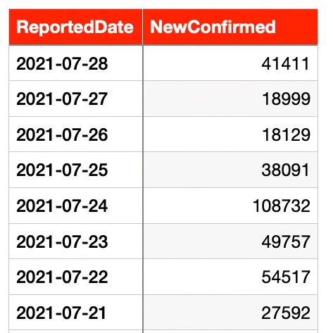
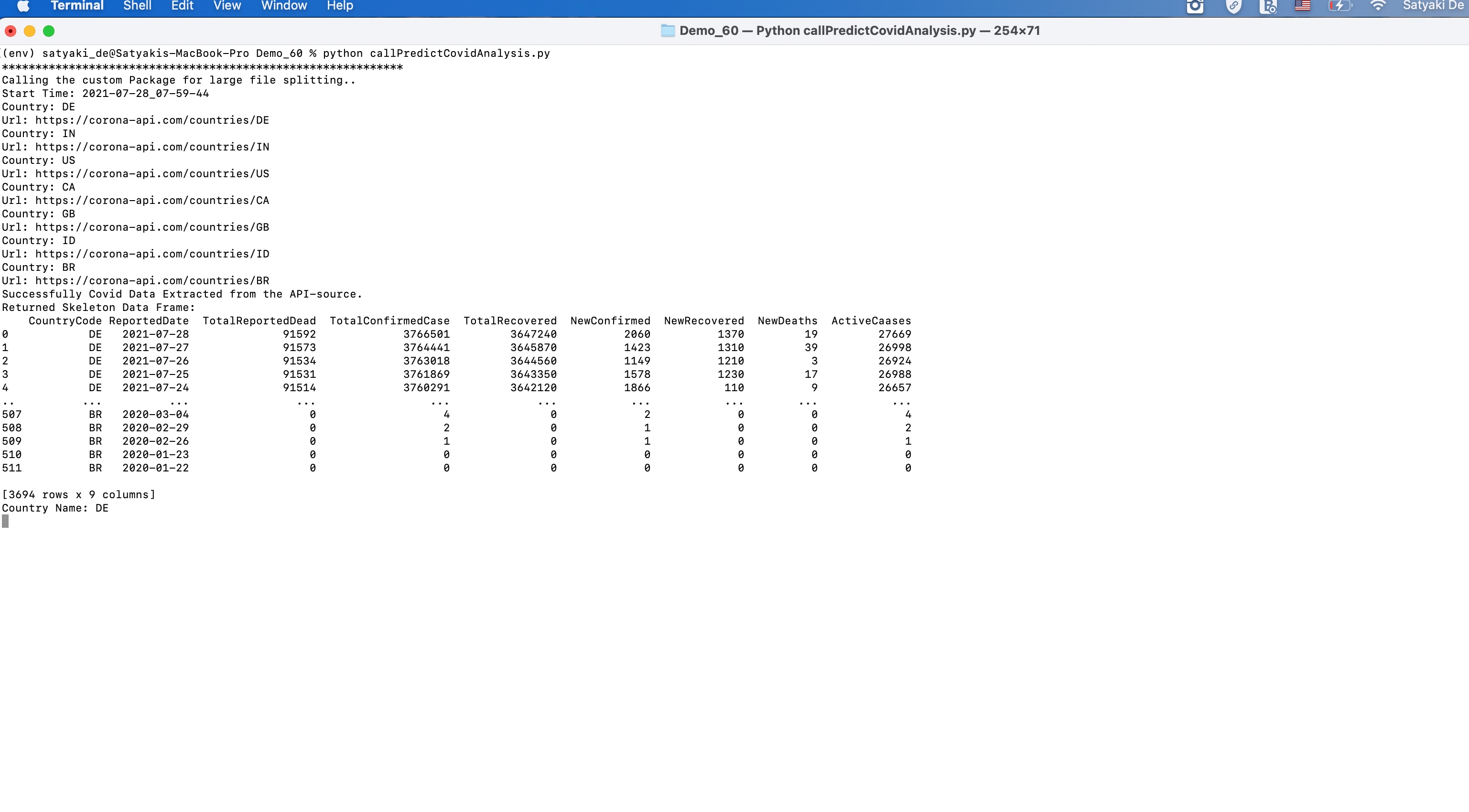
Let’s check one such use case since our source has plenty of good data points to decide. We’ve daily data of newly infected covid patients based on countries, as shown below –
Covid Cases
And, our clean class will transform the data into two fields –
Transformed Data
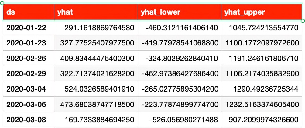
Once we fit the data into the prophet model, it will generate some additional columns, which will be used for prediction as shown below –
Generated data from prophet-api
And, a sample prediction based on a similar kind of data would be identical to this –
Sample Prediction
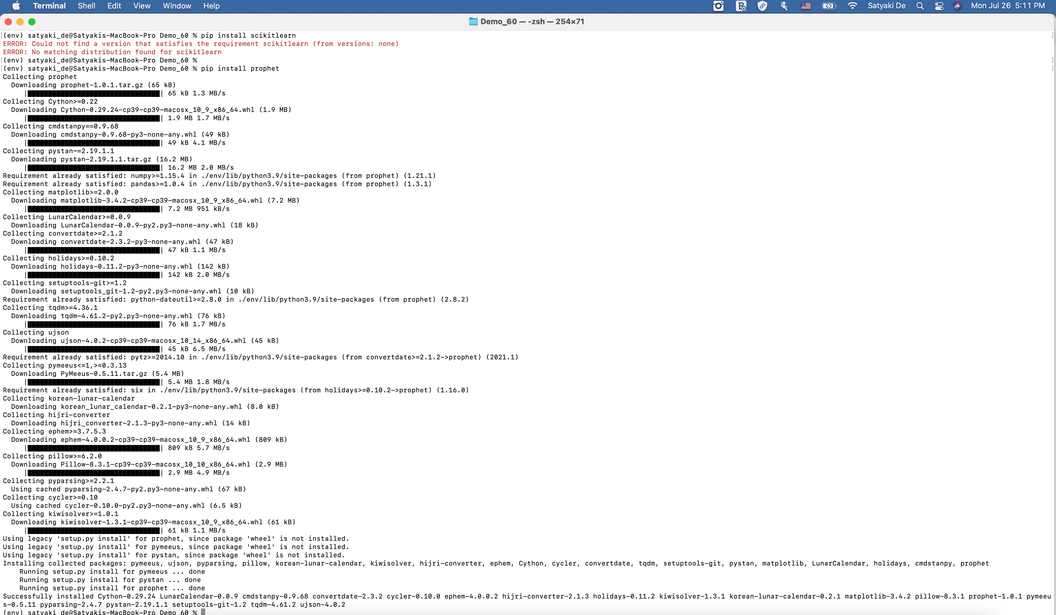
Let us understand what packages we need to install to prepare this application –
Installing Dependency Packages – IInstalling Dependency Packages – II
1. clsConfig.py ( This native Python script contains the configuration entries. )
This file contains hidden or bidirectional Unicode text that may be interpreted or compiled differently than what appears below. To review, open the file in an editor that reveals hidden Unicode characters. Learn more about bidirectional Unicode characters
We’re not going to discuss anything specific to this script.
2. clsL.py ( This native Python script logs the application. )
This file contains hidden or bidirectional Unicode text that may be interpreted or compiled differently than what appears below. To review, open the file in an editor that reveals hidden Unicode characters. Learn more about bidirectional Unicode characters
Based on the operating system, the log class will capture potential information under the “log” directory in the form of csv for later reference purposes.
3. clsForecast.py ( This native Python script will clean & transform the data. )
This file contains hidden or bidirectional Unicode text that may be interpreted or compiled differently than what appears below. To review, open the file in an editor that reveals hidden Unicode characters. Learn more about bidirectional Unicode characters
Let’s explore the critical snippet out of this script –
df_Comm = dfWork[[tms, fnc]]
Now, the application will extract only the relevant columns to proceed.
df_Comm.columns = ['ds', 'y']
It is now assigning specific column names, which is a requirement for prophet API.
4. clsCovidAPI.py ( This native Python script will call the Covid-19 API. )
This file contains hidden or bidirectional Unicode text that may be interpreted or compiled differently than what appears below. To review, open the file in an editor that reveals hidden Unicode characters. Learn more about bidirectional Unicode characters
The application will extract the elements & normalize the JSON & convert that to a pandas dataframe & also added one dummy column, which will use for the later purpose to merge the data from another set.
Now, the application will take the nested element & normalize that as per granular level. Also, it added the dummy column to join both of these data together.
The application will Merge both the data sets to get the complete denormalized data for our use cases.
# Merging with the previous Country Code data
if cnt == 0:
    df_M = df_fin
else:
    d_frames = [df_M, df_fin]
    df_M = p.concat(d_frames)
This entire deserializing execution happens per country. Hence, the above snippet will create an individual sub-group based on the country & later does union to all the sets.
If any calls to source API fails, the application will retrigger after waiting for a specific time until it reaches its maximum capacity.
5. callPredictCovidAnalysis.py ( This native Python script is the main one to predict the Covid. )
This file contains hidden or bidirectional Unicode text that may be interpreted or compiled differently than what appears below. To review, open the file in an editor that reveals hidden Unicode characters. Learn more about bidirectional Unicode characters
The application is extracting the full country name based on ISO country code.
# Lowercase the column names
iDF.columns = [c.lower() for c in iDF.columns]
# Determine which is Y axis
y_col = [c for c in iDF.columns if c.startswith('y')][0]
# Determine which is X axis
x_col = [c for c in iDF.columns if c.startswith('ds')][0]

# Data Conversion
iDF['y'] = iDF[y_col].astype('float')
iDF['ds'] = iDF[x_col].astype('datetime64[ns]')
The above script will convert all the column names in lower letters & then convert & cast them with the appropriate data type.
# Forecast calculations
# Decreasing the changepoint_prior_scale to 0.001 to make the trend less flexible
m = Prophet(n_changepoints=20, yearly_seasonality=True, changepoint_prior_scale=0.001)
m.fit(iDF)

forecastDF = m.make_future_dataframe(periods=365)

forecastDF = m.predict(forecastDF)

l.logr('15.forecastDF_' + var + '_' + countryCD + '.csv', debug_ind, forecastDF, 'log')

df_M = forecastDF[['ds', 'yhat', 'yhat_lower', 'yhat_upper']]

l.logr('16.df_M_' + var + '_' + countryCD + '.csv', debug_ind, df_M, 'log')
The above snippet will use the machine-learning driven prophet-API, where the application will fit the model & then predict based on the existing data for a year. Also, we’ve identified the number of changepoints. By default, the prophet-API adds 25 changepoints to the initial 80% of the data set that trend is less flexible.
Prophet allows you to adjust the trend in case there is an overfit or underfit. changepoint_prior_scale helps adjust the strength of the movement & decreasing the changepoint_prior_scale to 0.001 to make it less flexible.
The application is fetching & creating the country-specific dataframe.
for i in countryList:
    try:
        cntryIndiv = i.strip()

        print('Country Porcessing: ' + str(cntryIndiv))

        # Creating dataframe for each country
        # Germany Main DataFrame
        dfCountry = countrySpecificDF(df, cntryIndiv)
        l.logr(str(cnt) + '.df_' + cntryIndiv + '_' + var1 + '.csv', DInd, dfCountry, 'log')

        # Let's pass this to our map section
        retDFGenNC = x2.forecastNewConfirmed(dfCountry, DInd, var1)

        statVal = str(NC)

        a1 = plot_picture(retDFGenNC, DInd, var1, cntryIndiv, statVal)

        retDFGenNC_D = x2.forecastNewDead(dfCountry, DInd, var1)

        statVal = str(ND)

        a2 = plot_picture(retDFGenNC_D, DInd, var1, cntryIndiv, statVal)

        cntryFullName = countryDet(cntryIndiv)

        if (a1 + a2) == 0:
            oprMsg = cntryFullName + ' ' + SM
            print(oprMsg)
        else:
            oprMsg = cntryFullName + ' ' + FM
            print(oprMsg)

        # Resetting the dataframe value for the next iteration
        dfCountry = p.DataFrame()
        cntryIndiv = ''
        oprMsg = ''
        cntryFullName = ''
        a1 = 0
        a2 = 0
        statVal = ''

        cnt += 1
    except Exception as e:
        x = str(e)
        print(x)
The above snippet will call the function to predict the data & then predict the visual representation based on plotting the data points.
Let us run the application –
Application Run
And, it will generate the visual representation as follows –
Application Run – Continue
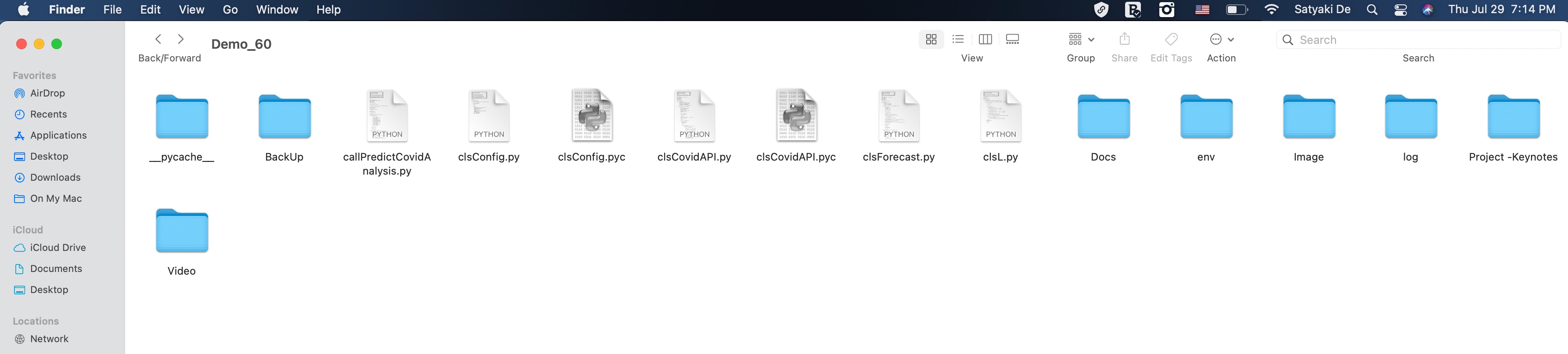
And, here is the folder structure –
Directory Structure
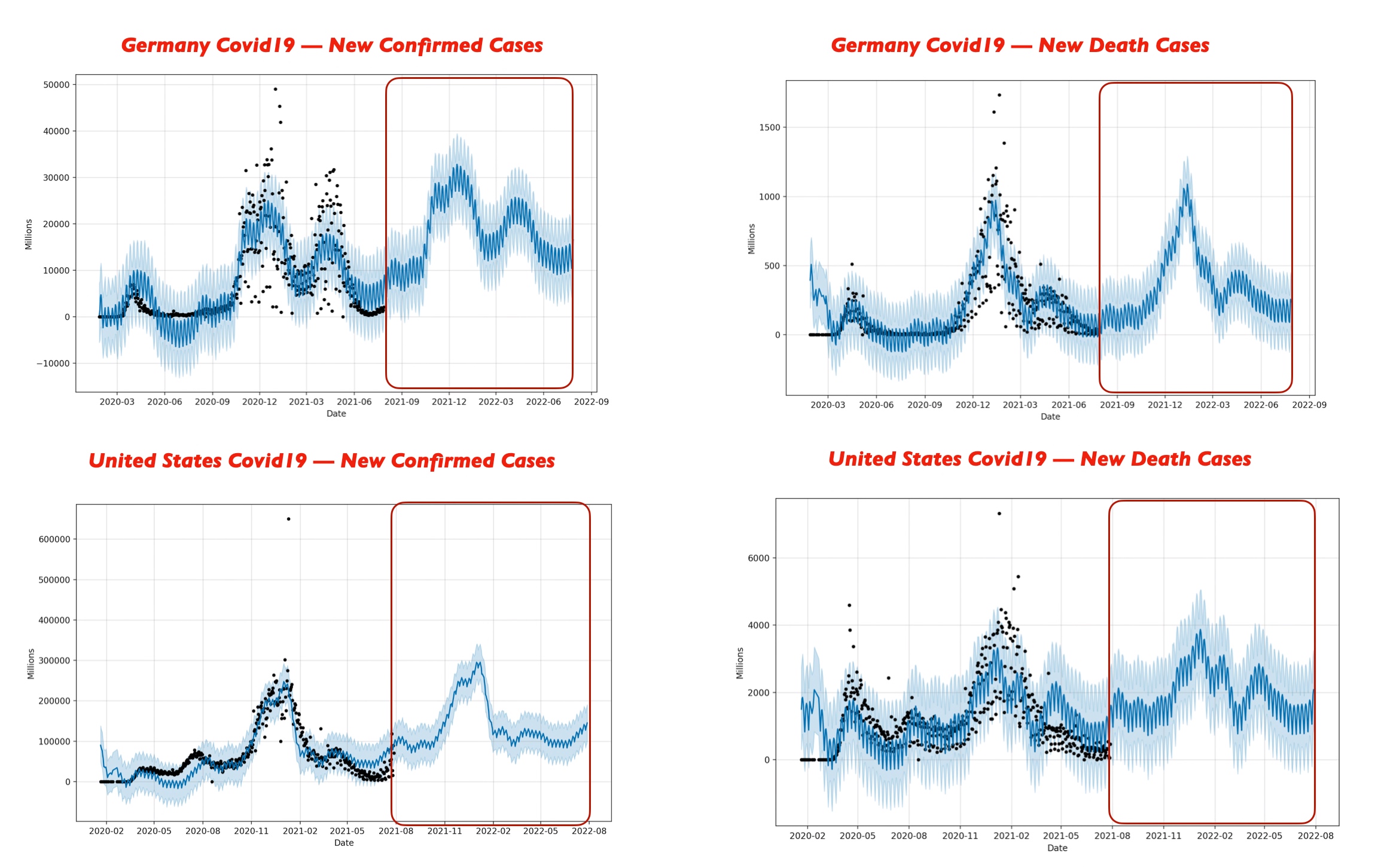
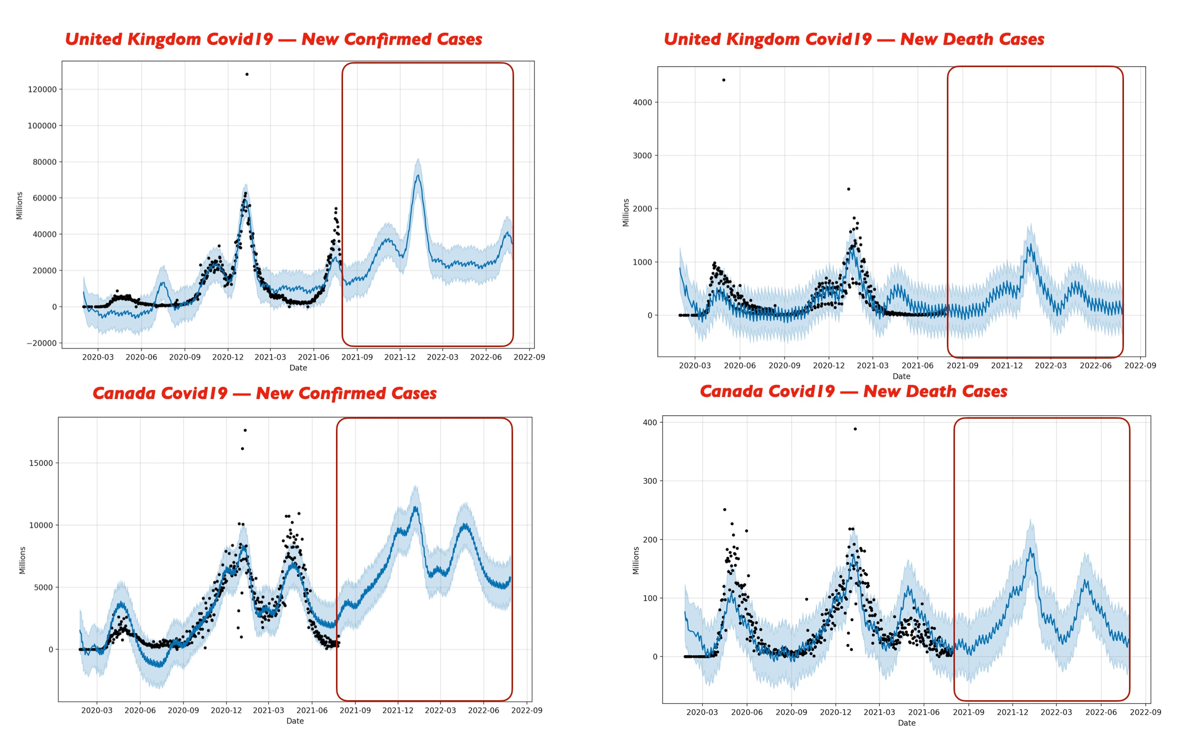
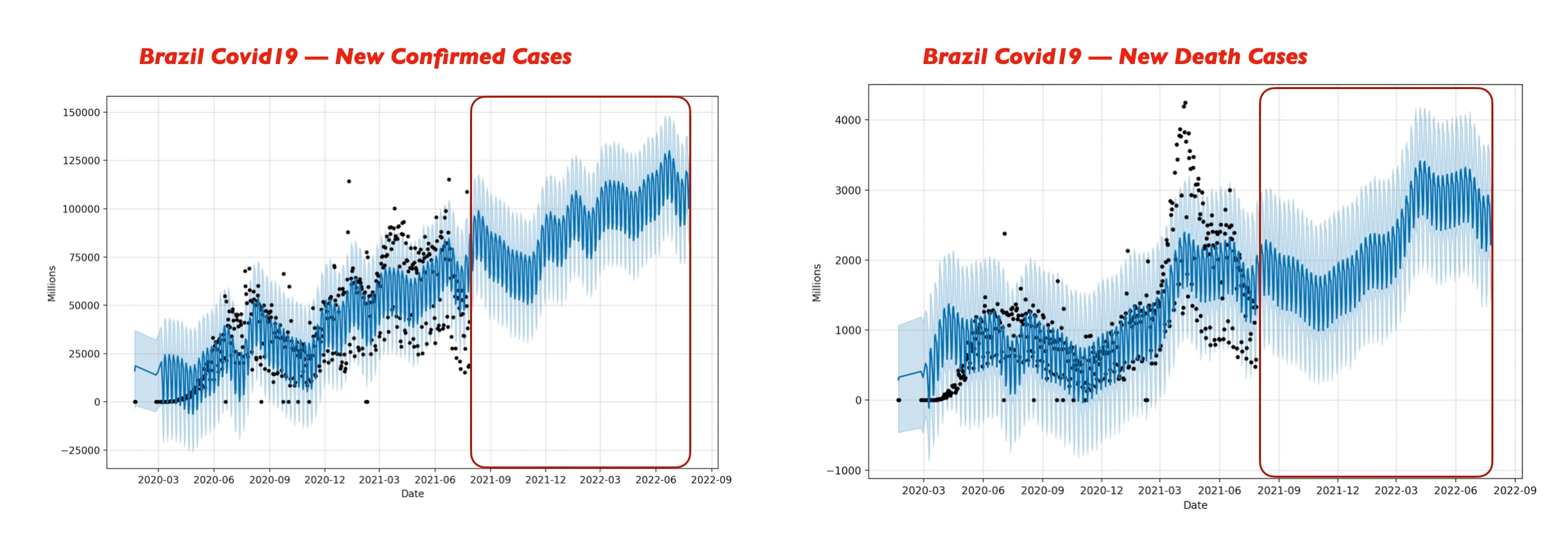
Let’s explore the comparison study & try to find out the outcome –
Option – 1
Option – 2
Option – 3
Option -4
Let us analyze from the above visual data-point.
Conclusion:
Let’s explore the comparison study & try to find out the outcome –
India may see a rise of new covid cases & it might cross the mark 400,000 during June 2022 & would be the highest among the countries that we’ve considered here including India, Indonesia, Germany, US, UK, Canada & Brazil. The second worst affected country might be the US during the same period. The third affected country will be Indonesia during the same period.
Canada will be the least affected country during June 2022. The figure should be within 12,000.
However, death case wise India is not only the leading country. The US, India & Brazil will see almost 4000 or slightly over the 4000 marks.
So, we’ve done it.
You will get the complete codebase in the following Github link.
I’ll bring some more exciting topic in the coming days from the Python verse.
Till then, Happy Avenging! 😀
Note: All the data & scenario posted here are representational data & scenarios & available over the internet & for educational purpose only.
One more thing you need to understand is that this prediction based on limited data points. The actual event may happen differently. Ideally, countries are taking a cue from this kind of analysis & are initiating appropriate measures to avoid the high-curve. And, that is one of the main objective of time series analysis.
There is always a room for improvement of this kind of models & the solution associated with it. I’ve shown the basic ways to achieve the same for the education purpose only.
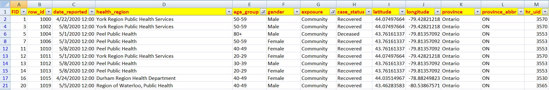
Today, I’ll be demonstrating some scenarios based on open-source data from Canada. In this post, I will only explain some of the significant parts of the code. Not the entire range of scripts here.
Let’s explore a couple of sample source data –
I would like to explore how much this disease caused an impact on the elderly in Canada.
Let’s explore the source directory structure –
For this, you need to install the following packages –
In this case, we’ve downloaded the data from Canada’s site. However, they have created API. So, you can consume the data through that way as well. Since the volume is a little large. I decided to download that in CSV & then use that for my analysis.
Before I start, let me explain a couple of critical assumptions that I had to make due to data impurities or availabilities.
If there is no data available for a specific case, my application will consider that patient as COVID-Active.
We will consider the patient is affected through Community-spreading until we have data to find it otherwise.
If there is no data available for gender, we’re marking these records as “Other.” So, that way, we’re making it into that category, where the patient doesn’t want to disclose their sexual orientation.
If we don’t have any data, then by default, the application is considering the patient is alive.
Lastly, my application considers the middle point of the age range data for all the categories, i.e., the patient’s age between 20 & 30 will be considered as 25.
1. clsCovidAnalysisByCountryAdv (This is the main script, which will invoke the Machine-Learning API & return 0 if successful.)
################################################## Written By: SATYAKI DE ######## Written On: 01-Jun-2020 ######## Modified On 01-Jun-2020 ######## ######## Objective: Main scripts for Logistic ######## Regression. ##################################################importpandasaspimportclsLaslogimportdatetimeimportmatplotlib.pyplotaspltimportseabornassnsfromclsConfigimport clsConfig as cf
# %matplotlib inline -- for Jupyter NotebookclassclsCovidAnalysisByCountryAdv:
def__init__(self):
self.fileName_1 = cf.config['FILE_NAME_1']
self.fileName_2 = cf.config['FILE_NAME_2']
self.Ind = cf.config['DEBUG_IND']
self.subdir =str(cf.config['LOG_DIR_NAME'])
defsetDefaultActiveCases(self, row):
try:
str_status =str(row['case_status'])
if str_status =='Not Reported':
return'Active'else:
return str_status
except:
return'Active'defsetDefaultExposure(self, row):
try:
str_exposure =str(row['exposure'])
if str_exposure =='Not Reported':
return'Community'else:
return str_exposure
except:
return'Community'defsetGender(self, row):
try:
str_gender =str(row['gender'])
if str_gender =='Not Reported':
return'Other'else:
return str_gender
except:
return'Other'defsetSurviveStatus(self, row):
try:
# 0 - Deceased# 1 - Alive
str_active =str(row['ActiveCases'])
if str_active =='Deceased':
return0else:
return1except:
return1defgetAgeFromGroup(self, row):
try:
# We'll take the middle of the Age group# If a age range falls with 20, we'll# consider this as 10.# Similarly, a age group between 20 & 30,# should reflect by 25.# Anything above 80 will be considered as# 85
str_age_group =str(row['AgeGroup'])
if str_age_group =='<20':
return10elif str_age_group =='20-29':
return25elif str_age_group =='30-39':
return35elif str_age_group =='40-49':
return45elif str_age_group =='50-59':
return55elif str_age_group =='60-69':
return65elif str_age_group =='70-79':
return75else:
return85except:
return100defpredictResult(self):
try:
# Initiating Logging Instances
clog = log.clsL()
# Important variables
var = datetime.datetime.now().strftime(".%H.%M.%S")
print('Target File Extension will contain the following:: ', var)
Ind =self.Ind
subdir =self.subdir
######################################## ## Using Logistic Regression to ## Idenitfy the following scenarios - ## ## Age wise Infection Vs Deaths ## ########################################
inputFileName_2 =self.fileName_2
# Reading from Input File
df_2 = p.read_csv(inputFileName_2)
# Fetching only relevant columns
df_2_Mod = df_2[['date_reported','age_group','gender','exposure','case_status']]
df_2_Mod['State'] = df_2['province_abbr']
print()
print('Projecting 2nd file sample rows: ')
print(df_2_Mod.head())
print()
x_row_1 = df_2_Mod.shape[0]
x_col_1 = df_2_Mod.shape[1]
print('Total Number of Rows: ', x_row_1)
print('Total Number of columns: ', x_col_1)
########################################################################################## Few Assumptions ########################################################################################### By default, if there is no data on exposure - We'll treat that as community spreading ## By default, if there is no data on case_status - We'll consider this as active ## By default, if there is no data on gender - We'll put that under a separate Gender ## category marked as the "Other". This includes someone who doesn't want to identify ## his/her gender or wants to be part of LGBT community in a generic term. ## ## We'll transform our data accordingly based on the above logic. ##########################################################################################
df_2_Mod['ActiveCases'] = df_2_Mod.apply(lambda row: self.setDefaultActiveCases(row), axis=1)
df_2_Mod['ExposureStatus'] = df_2_Mod.apply(lambda row: self.setDefaultExposure(row), axis=1)
df_2_Mod['Gender'] = df_2_Mod.apply(lambda row: self.setGender(row), axis=1)
# Filtering all other records where we don't get any relevant information# Fetching Data for
df_3 = df_2_Mod[(df_2_Mod['age_group'] !='Not Reported')]
# Dropping unwanted columns
df_3.drop(columns=['exposure'], inplace=True)
df_3.drop(columns=['case_status'], inplace=True)
df_3.drop(columns=['date_reported'], inplace=True)
df_3.drop(columns=['gender'], inplace=True)
# Renaming one existing column
df_3.rename(columns={"age_group": "AgeGroup"}, inplace=True)
# Creating important feature# 0 - Deceased# 1 - Alive
df_3['Survived'] = df_3.apply(lambda row: self.setSurviveStatus(row), axis=1)
clog.logr('2.df_3'+ var +'.csv', Ind, df_3, subdir)
print()
print('Projecting Filter sample rows: ')
print(df_3.head())
print()
x_row_2 = df_3.shape[0]
x_col_2 = df_3.shape[1]
print('Total Number of Rows: ', x_row_2)
print('Total Number of columns: ', x_col_2)
# Let's do some basic checkings
sns.set_style('whitegrid')
#sns.countplot(x='Survived', hue='Gender', data=df_3, palette='RdBu_r')# Fixing Gender Column# This will check & indicate yellow for missing entries#sns.heatmap(df_3.isnull(), yticklabels=False, cbar=False, cmap='viridis')#sex = p.get_dummies(df_3['Gender'], drop_first=True)
sex = p.get_dummies(df_3['Gender'])
df_4 = p.concat([df_3, sex], axis=1)
print('After New addition of columns: ')
print(df_4.head())
clog.logr('3.df_4'+ var +'.csv', Ind, df_4, subdir)
# Dropping unwanted columns for our Machine Learning
df_4.drop(columns=['Gender'], inplace=True)
df_4.drop(columns=['ActiveCases'], inplace=True)
df_4.drop(columns=['Male','Other','Transgender'], inplace=True)
clog.logr('4.df_4_Mod'+ var +'.csv', Ind, df_4, subdir)
# Fixing Spread Columns
spread = p.get_dummies(df_4['ExposureStatus'], drop_first=True)
df_5 = p.concat([df_4, spread], axis=1)
print('After Spread columns:')
print(df_5.head())
clog.logr('5.df_5'+ var +'.csv', Ind, df_5, subdir)
# Dropping unwanted columns for our Machine Learning
df_5.drop(columns=['ExposureStatus'], inplace=True)
clog.logr('6.df_5_Mod'+ var +'.csv', Ind, df_5, subdir)
# Fixing Age Columns
df_5['Age'] = df_5.apply(lambda row: self.getAgeFromGroup(row), axis=1)
df_5.drop(columns=["AgeGroup"], inplace=True)
clog.logr('7.df_6'+ var +'.csv', Ind, df_5, subdir)
# Fixing Dummy Columns Name# Renaming one existing column Travel-Related with Travel_Related
df_5.rename(columns={"Travel-Related": "TravelRelated"}, inplace=True)
clog.logr('8.df_7'+ var +'.csv', Ind, df_5, subdir)
# Removing state for temporary basis
df_5.drop(columns=['State'], inplace=True)
# df_5.drop(columns=['State','Other','Transgender','Pending','TravelRelated','Male'], inplace=True)# Casting this entire dataframe into Integer# df_5_temp.apply(p.to_numeric)print('Info::')
print(df_5.info())
print("*"*60)
print(df_5.describe())
print("*"*60)
clog.logr('9.df_8'+ var +'.csv', Ind, df_5, subdir)
print('Intermediate Sample Dataframe for Age::')
print(df_5.head())
# Plotting it to Graphsns.jointplot(x="Age", y='Survived', data=df_5)
sns.jointplot(x="Age", y='Survived', data=df_5, kind='kde', color='red')
plt.xlabel("Age")
plt.ylabel("Data Point (0 - Died Vs 1 - Alive)")# Another check with Age Group
sns.countplot(x='Survived', hue='Age', data=df_5, palette='RdBu_r')
plt.xlabel("Survived(0 - Died Vs 1 - Alive)")
plt.ylabel("Total No Of Patient")
df_6 = df_5.drop(columns=['Survived'], axis=1)
clog.logr('10.df_9'+ var +'.csv', Ind, df_6, subdir)
# Train & Split Data
x_1 = df_6
y_1 = df_5['Survived']
# Now Train-Test Split of your source datafromsklearn.model_selectionimport train_test_split
# test_size => % of allocated data for your test cases# random_state => A specific set of random split on your data
X_train_1, X_test_1, Y_train_1, Y_test_1 = train_test_split(x_1, y_1, test_size=0.3, random_state=101)
# Importing Modelfromsklearn.linear_modelimport LogisticRegression
logmodel = LogisticRegression()
logmodel.fit(X_train_1, Y_train_1)
# Adding Predictions to it
predictions_1 = logmodel.predict(X_test_1)
fromsklearn.metricsimport classification_report
print('Classification Report:: ')
print(classification_report(Y_test_1, predictions_1))
fromsklearn.metricsimport confusion_matrix
print('Confusion Matrix:: ')
print(confusion_matrix(Y_test_1, predictions_1))
# This is require when you are trying to print from conventional# front & not using Jupyter notebook.
plt.show()
return0exceptExceptionas e:
x =str(e)
print('Error : ', x)
return1
Key snippets from the above script –
df_2_Mod['ActiveCases'] = df_2_Mod.apply(lambda row: self.setDefaultActiveCases(row), axis=1)df_2_Mod['ExposureStatus'] = df_2_Mod.apply(lambda row: self.setDefaultExposure(row), axis=1)df_2_Mod['Gender'] = df_2_Mod.apply(lambda row: self.setGender(row), axis=1)# Filtering all other records where we don't get any relevant information# Fetching Data fordf_3 = df_2_Mod[(df_2_Mod['age_group'] != 'Not Reported')]# Dropping unwanted columnsdf_3.drop(columns=['exposure'], inplace=True)df_3.drop(columns=['case_status'], inplace=True)df_3.drop(columns=['date_reported'], inplace=True)df_3.drop(columns=['gender'], inplace=True)# Renaming one existing columndf_3.rename(columns={"age_group": "AgeGroup"}, inplace=True)# Creating important feature# 0 - Deceased# 1 - Alivedf_3['Survived'] = df_3.apply(lambda row: self.setSurviveStatus(row), axis=1)
The above lines point to the critical transformation areas, where the application is invoking various essential business logic.
The above lines will transform the data into this –
As you can see, we’ve transformed the row values into columns with binary values. This kind of transformation is beneficial.
# Plotting it to Graphsns.jointplot(x="Age", y='Survived', data=df_5)sns.jointplot(x="Age", y='Survived', data=df_5, kind='kde', color='red')plt.xlabel("Age")plt.ylabel("Data Point (0 - Died Vs 1 - Alive)")# Another check with Age Groupsns.countplot(x='Survived', hue='Age', data=df_5, palette='RdBu_r')plt.xlabel("Survived(0 - Died Vs 1 - Alive)")plt.ylabel("Total No Of Patient")
The above lines will process the data & visualize based on that.
x_1 = df_6y_1 = df_5['Survived']
In the above snippet, we’ve assigned the features & target variable for our final logistic regression model.
# Now Train-Test Split of your source datafrom sklearn.model_selection import train_test_split# test_size => % of allocated data for your test cases# random_state => A specific set of random split on your dataX_train_1, X_test_1, Y_train_1, Y_test_1 = train_test_split(x_1, y_1, test_size=0.3, random_state=101)# Importing Modelfrom sklearn.linear_model import LogisticRegressionlogmodel = LogisticRegression()logmodel.fit(X_train_1, Y_train_1)
In the above snippet, we’re splitting the primary data & create a set of test & train data. Once we have the collection, the application will put the logistic regression model. And, finally, we’ll fit the training data.
The above lines, finally use the model & then we feed our test data.
Let’s see how it runs –
And, here is the log directory –
For better understanding, I’m just clubbing both the diagram at one place & the final outcome is showing as follows –
So, from the above picture, we can see that the maximum vulnerable patients are patients who are 80+. The next two categories that also suffered are 70+ & 60+.
Also, We’ve checked the Female Vs. Male in the following code –
sns.countplot(x='Survived', hue='Female', data=df_5, palette='RdBu_r')plt.xlabel("Survived(0 - Died Vs 1 - Alive)")plt.ylabel("Female Vs Male (Including Other Genders)")
And, the analysis represents through this –
In this case, you have to consider that the Male part includes all the other genders apart from the actual Male. Hence, I believe death for females would be more compared to people who identified themselves as males.
So, finally, we’ve done it.
During this challenging time, I would request you to follow strict health guidelines & stay healthy.
N.B.: All the data that are used here can be found in the public domain. We use this solely for educational purposes. You can find the details here.


You must be logged in to post a comment.