This site mainly deals with various use cases demonstrated using Python, Data Science, Cloud basics, SQL Server, Oracle, Teradata along with SQL & their implementation. Expecting yours active participation & time. This blog can be access from your TP, Tablet & mobile also. Please provide your feedback.
This is a continuation of my previous post, which can be found here.
Let us recap the key takaways from our previous post –
Agentic AI refers to autonomous systems that pursue goals with minimal supervision by planning, reasoning about next steps, utilizing tools, and maintaining context across sessions. Core capabilities include goal-directed autonomy, interaction with tools and environments (e.g., APIs, databases, devices), multi-step planning and reasoning under uncertainty, persistence, and choiceful decision-making.
Architecturally, three modules coordinate intelligent behavior: Sensing (perception pipelines that acquire multimodal data, extract salient patterns, and recognize entities/events); Observation/Deliberation (objective setting, strategy formation, and option evaluation relative to resources and constraints); and Action (execution via software interfaces, communications, or physical actuation to deliver outcomes). These functions are enabled by machine learning, deep learning, computer vision, natural language processing, planning/decision-making, uncertainty reasoning, and simulation/modeling.
At enterprise scale, open standards align autonomy with governance: the Model Context Protocol (MCP) grants an agent secure, principled access to enterprise tools and data (vertical integration), while Agent-to-Agent (A2A) enables specialized agents to coordinate, delegate, and exchange information (horizontal collaboration). Together, MCP and A2A help organizations transition from isolated pilots to scalable programs, delivering end-to-end automation, faster integration, enhanced security and auditability, vendor-neutral interoperability, and adaptive problem-solving that responds to real-time context.
Great! Let’s dive into this topic now.
Enterprise AI with MCP refers to the application of the Model Context Protocol (MCP), an open standard, to enable AI systems to securely and consistently access external enterprise data and applications.
The problem MCP solves in enterprise AI:
Before MCP, enterprise AI integration was characterized by a “many-to-many” or “N x M” problem. Companies had to build custom, fragile, and costly integrations between each AI model and every proprietary data source, which was not scalable. These limitations left AI agents with limited, outdated, or siloed information, restricting their potential impact. MCP addresses this by offering a standardized architecture for AI and data systems to communicate with each other.
How does MCP work?
The MCP framework uses a client-server architecture to enable communication between AI models and external tools and data sources.
MCP Host: The AI-powered application or environment, such as an AI-enhanced IDE or a generative AI chatbot like Anthropic’s Claude or OpenAI’s ChatGPT, where the user interacts.
MCP Client: A component within the host application that manages the connection to MCP servers.
MCP Server: A lightweight service that wraps around an external system (e.g., a CRM, database, or API) and exposes its capabilities to the AI client in a standardized format, typically using JSON-RPC 2.0.
An MCP server provides AI clients with three key resources:
Resources: Structured or unstructured data that an AI can access, such as files, documents, or database records.
Tools: The functionality to perform specific actions within an external system, like running a database query or sending an email.
Prompts: Pre-defined text templates or workflows to help guide the AI’s actions.
Benefits of MCP for enterprise AI:
Standardized integration: Developers can build integrations against a single, open standard, which dramatically reduces the complexity and time required to deploy and scale AI initiatives.
Enhanced security and governance: MCP incorporates native support for security and compliance measures. It provides permission models, access control, and auditing capabilities to ensure AI systems only access data and tools within specified boundaries.
Real-time contextual awareness: By connecting AI agents to live enterprise data sources, MCP ensures they have access to the most current and relevant information, which reduces hallucinations and improves the accuracy of AI outputs.
Greater interoperability: MCP is model-agnostic & can be used with a variety of AI models (e.g., Anthropic’s Claude or OpenAI’s models) and across different cloud environments. This approach helps enterprises avoid vendor lock-in.
Accelerated development: The “build once, integrate everywhere” approach enables internal teams to focus on innovation instead of writing custom connectors for every system.
Flow of activities:
Let us understand one sample case & the flow of activities.
A customer support agent uses an AI assistant to get information about a customer’s recent orders. The AI assistant utilizes an MCP-compliant client to communicate with an MCP server, which is connected to the company’s PostgreSQL database.
The interaction flow:
1. User request: The support agent asks the AI assistant, “What was the most recent order placed by Priyanka Chopra Jonas?”
2. AI model processes intent: The AI assistant, running on an MCP host, analyzes the natural language query. It recognizes that to answer this question, it needs to perform a database query. It then identifies the appropriate tool from the MCP server’s capabilities.
3. Client initiates tool call: The AI assistant’s MCP client sends a JSON-RPC request to the MCP server connected to the PostgreSQL database. The request specifies the tool to be used, such as get_customer_orders, and includes the necessary parameters:
5. Database returns data: The PostgreSQL database executes the query and returns the requested data to the MCP server.
6. Server formats the response: The MCP server receives the raw database output and formats it into a standardized JSON response that the MCP client can understand.
7. Client returns data to the model: The MCP client receives the JSON response and passes it back to the AI assistant’s language model.
8. AI model generates final response: The language model incorporates this real-time data into its response and presents it to the user in a natural, conversational format.
“Priyanka Chopra Jonas’s most recent order was placed on August 25, 2025, with an order ID of 98765, for a total of $11025.50.”
What are the performance implications of using MCP for database access?
Using the Model Context Protocol (MCP) for database access introduces a layer of abstraction that affects performance in several ways. While it adds some latency and processing overhead, strategic implementation can mitigate these effects. For AI applications, the benefits often outweigh the costs, particularly in terms of improved accuracy, security, and scalability.
Sources of performance implications::
Added latency and processing overhead:
The MCP architecture introduces extra communication steps between the AI agent and the database, each adding a small amount of latency.
RPC overhead: The JSON-RPC call from the AI’s client to the MCP server adds a small processing and network delay. This is an out-of-process request, as opposed to a simple local function call.
JSON serialization: Request and response data must be serialized and deserialized into JSON format, which requires processing time.
Network transit: For remote MCP servers, the data must travel over the network, adding latency. However, for a local or on-premise setup, this is minimal. The physical location of the MCP server relative to the AI model and the database is a significant factor.
Scalability and resource consumption:
The performance impact scales with the complexity and volume of the AI agent’s interactions.
High request volume: A single AI agent working on a complex task might issue dozens of parallel database queries. In high-traffic scenarios, managing numerous simultaneous connections can strain system resources and require robust infrastructure.
Excessive data retrieval: A significant performance risk is an AI agent retrieving a massive dataset in a single query. This process can consume a large number of tokens, fill the AI’s context window, and cause bottlenecks at the database and client levels.
Context window usage: Tool definitions and the results of tool calls consume space in the AI’s context window. If a large number of tools are in use, this can limit the AI’s “working memory,” resulting in slower and less effective reasoning.
Optimizations for high performance::
Caching:
Caching is a crucial strategy for mitigating the performance overhead of MCP.
In-memory caching: The MCP server can cache results from frequent or expensive database queries in memory (e.g., using Redis or Memcached). This approach enables repeat requests to be served almost instantly without requiring a database hit.
Semantic caching: Advanced techniques can cache the results of previous queries and serve them for semantically similar future requests, reducing token consumption and improving speed for conversational applications.
Efficient queries and resource management:
Designing the MCP server and its database interactions for efficiency is critical.
Optimized SQL: The MCP server should generate optimized SQL queries. Database indexes should be utilized effectively to expedite lookups and minimize load.
Pagination and filtering: To prevent a single query from overwhelming the system, the MCP server should implement pagination. The AI agent can be prompted to use filtering parameters to retrieve only the necessary data.
Connection pooling: This technique reuses existing database connections instead of opening a new one for each request, thereby reducing latency and database load.
Load balancing and scaling:
For large-scale enterprise deployments, scaling is essential for maintaining performance.
Multiple servers: The workload can be distributed across various MCP servers. One server could handle read requests, and another could handle writes.
Load balancing: A reverse proxy or other load-balancing solution can distribute incoming traffic across MCP server instances. Autoscaling can dynamically add or remove servers in response to demand.
The performance trade-off in perspective:
For AI-driven tasks, a slight increase in latency for database access is often a worthwhile trade-off for significant gains.
Improved accuracy: Accessing real-time, high-quality data through MCP leads to more accurate and relevant AI responses, reducing “hallucinations”.
Scalable ecosystem: The standardization of MCP reduces development overhead and allows for a more modular, scalable ecosystem, which saves significant engineering resources compared to building custom integrations.
Decoupled architecture: The MCP server decouples the AI model from the database, allowing each to be optimized and scaled independently.
We’ll go ahead and conclude this post here & continue discussing on a further deep dive in the next post.
Till then, Happy Avenging! 🙂
Note: All the data & scenarios posted here are representational data & scenarios & available over the internet & for educational purposes only. There is always room for improvement in this kind of model & the solution associated with it. I’ve shown the basic ways to achieve the same for educational purposes only.
Today, we won’t be discussing any solutions. Today, we’ll be discussing the Agentic AI & its implementation in the Enterprise landscape in a series of upcoming posts.
So, hang tight! We’re about to launch a new venture as part of our knowledge drive.
What is Agentic AI?
Agentic AI refers to artificial intelligence systems that can act autonomously to achieve goals, making decisions and taking actions without constant human oversight. Unlike traditional AI, which responds to prompts, agentic AI can plan, reason about next steps, utilize tools, and work toward objectives over extended periods of time.
Key characteristics of agentic AI include:
Autonomy and Goal-Directed Behavior: These systems can pursue objectives independently, breaking down complex tasks into smaller steps and executing them sequentially.
Tool Use and Environment Interaction: Agentic AI can interact with external systems, APIs, databases, and software tools to gather information and perform actions in the real world.
Planning and Reasoning: They can develop multi-step strategies, adapt their approach based on feedback, and reason through problems to find solutions.
Persistence: Unlike single-interaction AI, agentic systems can maintain context and continue working on tasks across multiple interactions or sessions.
Decision Making: They can evaluate options, weigh trade-offs, and make choices about how to proceed when faced with uncertainty.
Foundational Elements of Agentic AI Architectures:
Agentic AI systems have several interconnected components that work together to enable intelligent behaviour. Each element plays a crucial role in the overall functioning of the AI system, and they must interact seamlessly to achieve desired outcomes. Let’s explore each of these components in more detail.
Sensing:
The sensing module serves as the AI’s eyes and ears, enabling it to understand its surroundings and make informed decisions. Think of it as the system that helps the AI “see” and “hear” the world around it, much like how humans use their senses.
Gathering Information: The system collects data from multiple sources, including cameras for visual information, microphones for audio, sensors for physical touch, and digital systems for data. This step provides the AI with a comprehensive understanding of what’s happening.
Making Sense of Data: Raw information from sensors can be messy and overwhelming. This component processes the data to identify the essential patterns and details that actually matter for making informed decisions.
Recognizing What’s Important: Utilizing advanced techniques such as computer vision (for images), natural language processing (for text and speech), and machine learning (for data patterns), the system identifies and understands objects, people, events, and situations within the environment.
This sensing capability enables AI systems to transition from merely following pre-programmed instructions to genuinely understanding their environment and making informed decisions based on real-world conditions. It’s the difference between a basic automated system and an intelligent agent that can adapt to changing situations.
Observation:
The observation module serves as the AI’s decision-making center, where it sets objectives, develops strategies, and selects the most effective actions to take. This step is where the AI transforms what it perceives into purposeful action, much like humans think through problems and devise plans.
Setting Clear Objectives: The system establishes specific goals and desired outcomes, giving the AI a clear sense of direction and purpose. This approach helps ensure all actions are working toward meaningful results rather than random activity.
Strategic Planning: Using information about its own capabilities and the current situation, the AI creates step-by-step plans to reach its goals. It considers potential obstacles, available resources, and different approaches to find the most effective path forward.
Intelligent Decision-Making: When faced with multiple options, the system evaluates each choice against the current circumstances, established goals, and potential outcomes. It then selects the action most likely to move the AI closer to achieving its objectives.
This observation capability is what transforms an AI from a simple tool that follows commands into an intelligent system that can work independently toward business goals. It enables the AI to handle complex, multi-step tasks and adapt its approach when conditions change, making it valuable for a wide range of applications, from customer service to project management.
Action:
The action module serves as the AI’s hands and voice, turning decisions into real-world results. This step is where the AI actually puts its thinking and planning into action, carrying out tasks that make a tangible difference in the environment.
Control Systems: The system utilizes various tools to interact with the world, including motors for physical movement, speakers for communication, network connections for digital tasks, and software interfaces for system operation. These serve as the AI’s means of reaching out and making adjustments.
Task Implementation: Once the cognitive module determines the action to take, this component executes the actual task. Whether it’s sending an email, moving a robotic arm, updating a database, or scheduling a meeting, this module handles the execution from start to finish.
This action capability is what makes AI systems truly useful in business environments. Without it, an AI could analyze data and make significant decisions, but it couldn’t help solve problems or complete tasks. The action module bridges the gap between artificial intelligence and real-world impact, enabling AI to automate processes, respond to customers, manage systems, and deliver measurable business value.
Technology that is primarily involved in the Agentic AI is as follows –
1. Machine Learning
2. Deep Learning
3. Computer Vision
4. Natural Language Processing (NLP)
5. Planning and Decision-Making
6. Uncertainty and Reasoning
7. Simulation and Modeling
Agentic AI at Scale: MCP + A2A:
In an enterprise setting, agentic AI systems utilize the Model Context Protocol (MCP) and the Agent-to-Agent (A2A) protocol as complementary, open standards to achieve autonomous, coordinated, and secure workflows. An MCP-enabled agent gains the ability to access and manipulate enterprise tools and data. At the same time, A2A allows a network of these agents to collaborate on complex tasks by delegating and exchanging information.
This combined approach allows enterprises to move from isolated AI experiments to strategic, scalable, and secure AI programs.
How do the protocols work together in an enterprise?
Protocol
Function in Agentic AI
Focus
Example use case
Model Context Protocol (MCP)
Equips a single AI agent with the tools and data it needs to perform a specific job.
Vertical integration: connecting agents to enterprise systems like databases, CRMs, and APIs.
A sales agent uses MCP to query the company CRM for a client’s recent purchase history.
Agent-to-Agent (A2A)
Enables multiple specialized agents to communicate, delegate tasks, and collaborate on a larger, multi-step goal.
Horizontal collaboration: allowing agents from different domains to work together seamlessly.
An orchestrating agent uses A2A to delegate parts of a complex workflow to specialized HR, IT, and sales agents.
Advantages for the enterprise:
End-to-end automation: Agents can handle tasks from start to finish, including complex, multi-step workflows, autonomously.
Greater agility and speed: Enterprise-wide adoption of these protocols reduces the cost and complexity of integrating AI, accelerating deployment timelines for new applications.
Enhanced security and governance: Enterprise AI platforms built on these open standards incorporate robust security policies, centralized access controls, and comprehensive audit trails.
Vendor neutrality and interoperability: As open standards, MCP and A2A allow AI agents to work together seamlessly, regardless of the underlying vendor or platform.
Adaptive problem-solving: Agents can dynamically adjust their strategies and collaborate based on real-time data and contextual changes, leading to more resilient and efficient systems.
We will discuss this topic further in our upcoming posts.
Till then, Happy Avenging! 🙂
Note: All the data & scenarios posted here are representational data & scenarios & available over the internet & for educational purposes only. There is always room for improvement in this kind of model & the solution associated with it. I’ve shown the basic ways to achieve the same for educational purposes only.
Today, we’re going to discuss creating a local LLM server and then utilizing it to execute various popular LLM models. We will club the local Apple GPUs together via a new framework that binds all the available Apple Silicon devices into one big LLM server. This enables people to run many large models, which was otherwise not possible due to the lack of GPUs.
This is certainly a new way; One can create virtual computation layers by adding nodes to the resource pool, increasing the computation capacity.
Why not witness a small demo to energize ourselves –
Let us understand the scenario. I’ve one Mac Book Pro M4 & 2 Mac Mini Pro M4 (Base models). So, I want to add them & expose them as a cluster as follows –
As you can see, I’ve connected my MacBook Pro with both the Mac Mini using high-speed thunderbolt cables for better data transmissions. And, I’ll be using an open-source framework called “Exo” to create it.
Also, you can see that my total computing capacity is 53.11 TFlops, which is slightly more than the last category.
What is Exo?
“Exo” is an open-source framework that helps you merge all your available devices into a large cluster of available resources. This extracts all the computing juice needed to handle complex tasks, including the big LLMs, which require very expensive GPU-based servers.
For more information on “Exo”, please refer to the following link.
In our previous diagram, we can see that the framework also offers endpoints.
One option is a local ChatGPT interface, where any question you ask will receive a response from models by combining all available computing power.
The other endpoint offers users a choice of any standard LLM API endpoint, which helps them integrate it into their solutions.
Let us see, how the devices are connected together –
How to establish the Cluster?
To proceed with this, you need to have at least Python 3.12, Anaconda or Miniconda & Xcode installed in all of your machines. Also, you need to install some Apple-specific MLX packages or libraries to get the best performance.
Depending on your choice, you need to use the following link to download Anaconda or Miniconda.
You can download the following link to download the Python 3.12. However, I’ve used Python 3.13 on some machines & some machines, I’ve used Python 3.12. And it worked without any problem.
Sometimes, after installing Anaconda or Miniconda, the environment may not implicitly be activated after successful installation. In that case, you may need to use the following commands in the terminal -> source ~/.bash_profile
To verify, whether the conda has been successfully installed & activated, you need to type the following command –
And, you need to perform the same process in other available devices as well.
Now, we’re ready to proceed with the final command –
(.venv) (exo1) satyaki_de@Satyakis-MacBook-Pro-Maxexo%exo/opt/anaconda3/envs/exo1/lib/python3.13/site-packages/google/protobuf/runtime_version.py:112: UserWarning:Protobufgencodeversion5.27.2isolderthantheruntimeversion5.28.1atnode_service.proto.Pleaseavoidchecked-inProtobufgencodethatcanbeobsolete.warnings.warn(NoneofPyTorch,TensorFlow>=2.0,orFlaxhavebeenfound.Modelswon't be available and only tokenizers, configuration and file/data utilities can be used.NoneofPyTorch,TensorFlow>=2.0,orFlaxhavebeenfound.Modelswon't be available and only tokenizers, configuration and file/data utilities can be used.Selectedinferenceengine: None__________/_ \ \//_ \ |__/>< (_) | \___/_/\_\___/Detectedsystem: AppleSiliconMacInferenceenginenameafterselection: mlxUsinginferenceengine: MLXDynamicShardInferenceEnginewithsharddownloader: SingletonShardDownloader[60771,54631,54661]Chatinterfacestarted:-http://127.0.0.1:52415-http://XXX.XXX.XX.XX:52415-http://XXX.XXX.XXX.XX:52415-http://XXX.XXX.XXX.XXX:52415ChatGPTAPIendpointservedat:-http://127.0.0.1:52415/v1/chat/completions-http://XXX.XXX.X.XX:52415/v1/chat/completions-http://XXX.XXX.XXX.XX:52415/v1/chat/completions-http://XXX.XXX.XXX.XXX:52415/v1/chat/completionshas_read=True,has_write=True╭────────────────────────────────────────────────────────────────────────────────────────────── ExoCluster (2nodes) ───────────────────────────────────────────────────────────────────────────────────────────────╮ReceivedexitsignalSIGTERM...Thankyouforusingexo.__________/_ \ \//_ \ |__/>< (_) | \___/_/\_\___/
Note that I’ve masked the IP addresses for security reasons.
Run Time:
At the beginning, if we trigger the main MacBook Pro Max, the “Exo” screen should looks like this –
And if you open the URL, you will see the following ChatGPT-like interface –
Connecting without the Thunderbolt bridge with the relevant port or a hub may cause performance degradation. Hence, how you connect will play a major role in the success of this intention. However, this is certainly a great idea to proceed with.
So, we’ve done it.
We’ll cover the detailed performance testing, Optimized configurations & many other useful details in our next post.
Till then, Happy Avenging! 🙂
Note: All the data & scenarios posted here are representational data & scenarios & available over the internet & for educational purposes only. There is always room for improvement in this kind of model & the solution associated with it. I’ve shown the basic ways to achieve the same for educational purposes only.
This new solution will evaluate the power of Stable Defussion, which is created solutions as we progress & refine our prompt from scratch by using Stable Defussion & Python. This post opens new opportunities for IT companies & business start-ups looking to deliver solutions & have better performance compared to the paid version of Stable Defussion AI’s API performance. This project is for the advanced Python, Stable Defussion for data Science Newbies & AI evangelists.
In a series of posts, I’ll explain and focus on the Stable Defussion API and custom solution using the Python-based SDK of Stable Defussion.
But, before that, let us view the video that it generates from the prompt by using the third-party API:
Prompt to Video
And, let us understand the prompt that we supplied to create the above video –
Lighthouse on a cliff overlooking the ocean, dynamic ocean waves crashing against rocks, dramatic clouds moving across sky, photorealistic water movement, mist and ocean spray, wind-driven waves, atmospheric sky motion, natural fluid dynamics, realistic, detailed, 8k. Do not change the size & shape of the lighthouse & the field on top of which the Lighthouse built.
Isn’t it exciting?
However, I want to stress this point: the video generated by the Stable Defusion (Stability AI) API was able to partially apply the animation effect. Even though the animation applies to the cloud, It doesn’t apply the animation to the wave. But, I must admit, the quality of the video is quite good.
Let us understand the code and how we run the solution, and then we can try to understand its performance along with the other solutions later in the subsequent series.
As you know, we’re exploring the code base of the third-party API, which will actually execute a series of API calls that create a video out of the prompt.
CODE:
Let us understand some of the important snippet –
classclsStabilityAIAPI:def__init__(self, STABLE_DIFF_API_KEY, OUT_DIR_PATH, FILE_NM, VID_FILE_NM):self.STABLE_DIFF_API_KEY = STABLE_DIFF_API_KEYself.OUT_DIR_PATH = OUT_DIR_PATHself.FILE_NM = FILE_NMself.VID_FILE_NM = VID_FILE_NMdefdelFile(self, fileName):try: # Deletingtheintermediateimageos.remove(fileName)return 0 exceptExceptionase:x = str(e)print('Error: ', x)return 1defgenerateText2Image(self, inputDescription):try:STABLE_DIFF_API_KEY = self.STABLE_DIFF_API_KEYfullFileName = self.OUT_DIR_PATH + self.FILE_NMifSTABLE_DIFF_API_KEYisNone:raiseException("MissingStabilityAPIkey.")response = requests.post(f"{api_host}/v1/generation/{engine_id}/text-to-image",headers={"Content-Type":"application/json","Accept":"application/json","Authorization":f"Bearer {STABLE_DIFF_API_KEY}"},json={"text_prompts": [{"text":inputDescription}],"cfg_scale":7,"height":1024,"width":576,"samples":1,"steps":30,},)ifresponse.status_code!=200:raiseException("Non-200 response: "+str(response.text))data=response.json()fori,imageinenumerate(data["artifacts"]):withopen(fullFileName,"wb") as f:f.write(base64.b64decode(image["base64"])) returnfullFileNameexceptExceptionas e:x=str(e)print('Error: ',x)return'N/A'defimage2VideoPassOne(self,imgNameWithPath):try:STABLE_DIFF_API_KEY=self.STABLE_DIFF_API_KEYresponse=requests.post(f"https://api.stability.ai/v2beta/image-to-video",headers={"authorization":f"Bearer {STABLE_DIFF_API_KEY}"},files={"image":open(imgNameWithPath,"rb")},data={"seed":0,"cfg_scale":1.8,"motion_bucket_id":127}, )print('First Pass Response:')print(str(response.text))genID=response.json().get('id')returngenIDexceptExceptionas e:x=str(e)print('Error: ',x)return'N/A'defimage2VideoPassTwo(self,genId):try:generation_id=genIdSTABLE_DIFF_API_KEY=self.STABLE_DIFF_API_KEYfullVideoFileName=self.OUT_DIR_PATH+self.VID_FILE_NMresponse=requests.request("GET",f"https://api.stability.ai/v2beta/image-to-video/result/{generation_id}",headers={'accept':"video/*", # Use 'application/json' to receive base64 encoded JSON'authorization':f"Bearer {STABLE_DIFF_API_KEY}"},) print('Retrieve Status Code: ',str(response.status_code))ifresponse.status_code==202:print("Generation in-progress, try again in 10 seconds.")return5elifresponse.status_code==200:print("Generation complete!")withopen(fullVideoFileName,'wb') as file:file.write(response.content)print("Successfully Retrieved the video file!")return0else:raiseException(str(response.json()))exceptExceptionas e:x=str(e)print('Error: ',x)return1
Now, let us understand the code –
1. CLASS INSTANTIATION
This function is called when an object of the class is created. It initializes four properties:
STABLE_DIFF_API_KEY: the API key for Stability AI services.
OUT_DIR_PATH: the folder path to save files.
FILE_NM: the name of the generated image file.
VID_FILE_NM: the name of the generated video file.
2. delFile(fileName)
This function deletes a file specified by fileName.
If successful, it returns 0.
If an error occurs, it logs the error and returns 1.
3. generateText2Image(inputDescription)
This function generates an image based on a text description:
Sends a request to the Stability AI text-to-image endpoint using the API key.
Saves the resulting image to a file.
Returns the file’s path on success or 'N/A' if an error occurs.
4. image2VideoPassOne(imgNameWithPath)
This function uploads an image to create a video in its first phase:
Sends the image to Stability AI’s image-to-video endpoint.
Logs the response and extracts the id (generation ID) for the next phase.
Returns the id if successful or 'N/A' on failure.
5. image2VideoPassTwo(genId)
This function retrieves the video created in the second phase using the genId:
Checks the video generation status from the Stability AI endpoint.
If complete, saves the video file and returns 0.
If still processing, returns 5.
Logs and returns 1 for any errors.
As you can see, the code is pretty simple to understand & we’ve taken all the necessary actions in case of any unforeseen network issues or even if the video is not ready after our job submission in the following lines of the main calling script (generateText2VideoAPI.py) –
Please let me know your feedback after reviewing all the posts! 🙂
Note: All the data & scenarios posted here are representational data & scenarios & available over the internet & for educational purposes only. There is always room for improvement in this kind of model & the solution associated with it. I’ve shown the basic ways to achieve the same for educational purposes only.
At the recent Argyle AI Summit, a prestigious event in the AI industry, I had the honor of participating as a speaker alongside esteemed professionals like Misha Leybovich from Google Labs. The summit, coordinated by Sylvia Das Chagas, a former senior AI conversation designer at CVS Health, provided an enlightening platform to discuss the evolving role of AI in talent management. Our session focused on the theme “Driving Talent with AI,” addressing some of the most pressing questions in the field. Frequently, relevant use cases were shared in detail to support these threads.
To view the actual page, please click the following link.
Impact of AI on Talent Management
One of the critical topics we explored was AI’s impact on talent management in the upcoming year. AI’s influence in hiring and retention is becoming increasingly significant. For example, AI-powered tools can now analyze vast amounts of data to identify the best candidates for a role, going beyond traditional resume screening. In retention, AI is instrumental in identifying patterns that indicate an employee’s likelihood to leave, enabling proactive measures.
Dispelling Fears Around AI Replacing Jobs
A burning question in AI is how leaders address fears that AI might replace manual jobs. We discussed the importance of leaders framing AI as a complement to human skills rather than a replacement. AI enhances employee capabilities by automating mundane tasks, allowing employees to focus on more creative and strategic work.
Innovative AI Tools for Organizations
Regarding new AI tools that organizations should watch out for, the conversation highlighted tools that enhance remote collaboration and workplace inclusivity. Tools like virtual meeting assistants that can transcribe, translate, and summarize meetings in real time are becoming invaluable in today’s global work environment.
AI in Boosting Employee Motivation and Productivity
AI’s role in boosting employee motivation and productivity was another focal point. We discussed how AI-driven career development programs can offer personalized learning paths, helping employees grow and stay motivated.
Incorporating Multilingual Capabilities in AI Tools
Incorporating multiple languages in tools like ChatGPT was highlighted as a critical step towards inclusivity. This expansion allows a broader range of employees to interact with AI tools in their native language, fostering a more inclusive workplace environment.
Addressing Reluctance to Change
Lastly, we tackled the challenge of addressing employees’ reluctance to change. Emphasizing the importance of transparent communication and education about AI’s benefits was identified as key. Organizations can alleviate fears and encourage a more accepting attitude towards AI by involving employees in the AI implementation process and providing training.
Conclusion
The Argyle AI Summit offered a compelling glimpse into the future of AI in talent management. The session provided valuable insights for leaders looking to harness AI’s potential to enhance talent management strategies by discussing real-world examples and strategies. To gain more in-depth knowledge and perspectives shared during this summit, I encourage interested parties to visit the recorded session link for a more comprehensive understanding.
Or, you can directly view it from here –
Feedback Request
I would greatly appreciate your feedback on the insights shared during the summit. Your thoughts and perspectives are invaluable as we continue to explore and navigate the evolving landscape of AI in the workplace.
Note: Video content hosted at a third-party site by the summit organizer & not by me.
Today, I’m going to discuss another Computer Vision installment. I’ll use Open CV & Kalman filter to predict a live ball movement of Cricket, one of the most popular sports in the Indian sub-continent, along with the UK & Australia. But before we start a deep dive, why don’t we first watch the demo?
Demo
Isn’t it exciting? Let’s explore it in detail.
Architecture:
Let us understand the flow of events –
The above diagram shows that the application, which uses Open CV, analyzes individual frames. It detects the cricket ball & finally, it tracks every movement by analyzing each frame & then it predicts (pink line) based on the supplied data points.
Python Packages:
Following are the python packages that are necessary to develop this brilliant use case –
Let us now understand the code. For this use case, we will only discuss three python scripts. However, we need more than these three. However, we have already discussed them in some of the early posts. Hence, we will skip them here.
clsPredictBodyLine.py (The main class that will handle the prediction of Cricket balls in the real-time video feed.)
This file contains hidden or bidirectional Unicode text that may be interpreted or compiled differently than what appears below. To review, open the file in an editor that reveals hidden Unicode characters. Learn more about bidirectional Unicode characters
Please find the key snippet from the above script –
kf = clsKalmanFilter()
The application is instantiating the modified Kalman filter.
myColorFinder = ColorFinder(False)
This command has more purpose than creating a proper mask in debug mode if you want to isolate the color of any object you want to track. To debug this property, one needs to set the flag to True. And you will see the following screen. Click the next video to get the process to generate the accurate HSV.
In the end, you will get a similar entry to the below one –
And you can see the entry that is available in the config for the following parameter –
The four points mentioned above will help us determine the best region for the ball, forcing the batsman to play the shots & a 90% chance of getting caught behind.
The snippets below will apply the mask & identify the contour of the objects which the program intends to track. In this case, we are talking about the pink cricket ball.
#Find the color ball
imgColor, mask = myColorFinder.update(img, hsvVals)

#Find location of the red_ball
imgContours, contours = cvzone.findContours(img, mask, minArea=500)

if contours:
    posListX.append(contours[0]['center'][0])
    posListY.append(contours[0]['center'][1])
The next key snippets are as follows –
if posListX:
    # Find the Coefficients
    A, B, C = np.polyfit(posListX, posListY, 2)

    for i, (posX, posY) in enumerate(zip(posListX, posListY)):
        pos = (posX, posY)
        cv2.circle(imgContours, pos, 10, (0,255,0), cv2.FILLED)

        # Using Karman Filter Prediction
        predicted = kf.predict(posX, posY)
        cv2.circle(imgContours, (predicted[0], predicted[1]), 12, (255,0,255), cv2.FILLED)

        ballDetectFlag = True
        if ballDetectFlag:
            print('Balls Detected!')

        if i == 0:
            cv2.line(imgContours, pos, pos, (0,255,0), 5)
            cv2.line(imgContours, predicted, predicted, (255,0,255), 5)
        else:
            predictedM = kf.predict(posListX[i-1], posListY[i-1])

            cv2.line(imgContours, pos, (posListX[i-1], posListY[i-1]), (0,255,0), 5)
            cv2.line(imgContours, predicted, predictedM, (255,0,255), 5)
The above lines will track the original & predicted lines & then it will plot on top of the frame in real time.
The next line will be as follows –
if len(posListX) < 10:

    # Calculation for best place to ball
    a1 = A
    b1 = B
    c1 = C - pT1

    X1 = int((- b1 - math.sqrt(b1**2 - (4*a1*c1)))/(2*a1))
    prediction1 = pT2 < X1 < pT3

    a2 = A
    b2 = B
    c2 = C - pT4

    X2 = int((- b2 - math.sqrt(b2**2 - (4*a2*c2)))/(2*a2))
    prediction2 = pT2 < X2 < pT3

    prediction = prediction1 | prediction2

if prediction:
    print('Good Length Ball!')
    sMsg = "Good Length Ball - (" + str(FrNo) + ")"
    cvzone.putTextRect(imgContours, sMsg, (50,150), scale=5, thickness=5, colorR=(0,200,0), offset=20)
else:
    print('Loose Ball!')
    sMsg = "Loose Ball - (" + str(FrNo) + ")"
    cvzone.putTextRect(imgContours, sMsg, (50,150), scale=5, thickness=5, colorR=(0,0,200), offset=20)
predictBodyLine.py (The main python script that will invoke the class to predict Cricket balls in the real-time video feed.)
This file contains hidden or bidirectional Unicode text that may be interpreted or compiled differently than what appears below. To review, open the file in an editor that reveals hidden Unicode characters. Learn more about bidirectional Unicode characters
# Passing source data csv file
x1 = pbdl.clsPredictBodyLine()

# Execute all the pass
r1 = x1.processVideo(debugInd, var)

if (r1 == 0):
    print('Successfully predicted body-line deliveries!')
else:
    print('Failed to predict body-line deliveries!')
The above lines will first instantiate the main class & then invoke it.
You can find it here if you want to know more about the Kalman filter.
So, finally, we’ve done it.
FOLDER STRUCTURE:
You will get the complete codebase in the following GitHub link.
I’ll bring some more exciting topics in the coming days from the Python verse. Please share & subscribe to my post & let me know your feedback.
Till then, Happy Avenging! 🙂
Note: All the data & scenarios posted here are representational data & scenarios & available over the internet & for educational purposes only. Some of the images (except my photo) we’ve used are available over the net. We don’t claim ownership of these images. There is always room for improvement & especially in the prediction quality.
This week we’re going to extend one of our earlier posts & trying to read an entire text from streaming using computer vision. If you want to view the previous post, please click the following link.
But, before we proceed, why don’t we view the demo first?
Demo
Architecture:
Let us understand the architecture flow –
Architecture flow
The above diagram shows that the application, which uses the Open-CV, analyzes individual frames from the source & extracts the complete text within the video & displays it on top of the target screen besides prints the same in the console.
Let us now understand the code. For this use case, we will only discuss three python scripts. However, we need more than these three. However, we have already discussed them in some of the early posts. Hence, we will skip them here.
clsReadingTextFromStream.py (This is the main class of python script that will extract the text from the WebCAM streaming in real-time.)
This file contains hidden or bidirectional Unicode text that may be interpreted or compiled differently than what appears below. To review, open the file in an editor that reveals hidden Unicode characters. Learn more about bidirectional Unicode characters
Please find the key snippet from the above script –
# Two output layer names for the text detector model

lNames = cf.conf['LAYER_DET']

# Tesseract OCR text param values

strVal = "-l " + str(cf.conf['LANG']) + " --oem " + str(cf.conf['OEM_VAL']) + " --psm " + str(cf.conf['PSM_VAL']) + ""
config = (strVal)
The first line contains the two output layers’ names for the text detector model. Among them, the first one indicates the outcome possibilities & the second one use to derive the bounding box coordinates of the predicted text.
The second line contains various options for the tesseract APIs. You need to understand the opportunities in detail to make them work. These are the essential options for our use case –
Language – The intended language, for example, English, Spanish, Hindi, Bengali, etc.
OEM flag – In this case, the application will use 4 to indicate LSTM neural net model for OCR.
OEM Value – In this case, the selected value is 7, indicating that the application treats the ROI as a single line of text.
For more details, please refer to the config file.
print("[INFO] Loading Text Detector...")
net = cv2.dnn.readNet(modelPath)
The above lines bring the already created model & load it to memory for evaluation.
# Setting new width and height and then determine the ratio in change
# for both the width and height
(newW, newH) = (wt, ht)
rW = origW / float(newW)
rH = origH / float(newH)

# Resize the frame and grab the new frame dimensions
frame = cv2.resize(frame, (newW, newH))
(H, W) = frame.shape[:2]

# Construct a blob from the frame and then perform a forward pass of
# the model to obtain the two output layer sets
blob = cv2.dnn.blobFromImage(frame, 1.0, (W, H), sParam, swapRB=True, crop=False)
net.setInput(blob)
(confScore, imgGeo) = net.forward(lNames)

# Decode the predictions, then apply non-maxima suppression to
# suppress weak, overlapping bounding boxes
(rects, confidences) = self.predictText(confScore, imgGeo)
boxes = non_max_suppression(np.array(rects), probs=confidences)
The above lines are more of preparing individual frames to get the bounding box by resizing the height & width followed by a forward pass of the model to obtain two output layer sets. And then apply the non-maxima suppression to remove the weak, overlapping bounding box by interpreting the prediction. In short, this will identify the potential text region & put the bounding box surrounding it.
# Initialize the list of results
res = []

# Getting BoundingBox boundaries
res = self.findBoundBox(boxes, res, rW, rH, orig, origW, origH, pad)
The above function will create the bounding box surrounding the predicted text regions. Also, we will capture the expected text inside the result variable.
for (spX, spY, epX, epY) in boxes:
  # Scale the bounding box coordinates based on the respective
  # ratios
  spX = int(spX * rW)
  spY = int(spY * rH)
  epX = int(epX * rW)
  epY = int(epY * rH)

  # To obtain a better OCR of the text we can potentially
  # apply a bit of padding surrounding the bounding box.
  # And, computing the deltas in both the x and y directions
  dX = int((epX - spX) * pad)
  dY = int((epY - spY) * pad)

  # Apply padding to each side of the bounding box, respectively
  spX = max(0, spX - dX)
  spY = max(0, spY - dY)
  epX = min(origW, epX + (dX * 2))
  epY = min(origH, epY + (dY * 2))

  # Extract the actual padded ROI
  roi = orig[spY:epY, spX:epX]
Now, the application will scale the bounding boxes based on the previously computed ratio for actual text recognition. In this process, the application also padded the bounding boxes & then extracted the padded region of interest.
# Choose the proper OCR Config
text = pytesseract.image_to_string(roi, config=config)

# Add the bounding box coordinates and OCR'd text to the list
# of results
res.append(((spX, spY, epX, epY), text))
Using OCR options, the application extracts the text within the video frame & adds that to the res list.
# Sort the results bounding box coordinates from top to bottom
res = sorted(res, key=lambda r:r[0][1])
It then sends a sorted output to the primary calling functions.
for ((spX, spY, epX, epY), text) in res:
  # Display the text OCR by using Tesseract APIs
  print("Reading Text::")
  print("=" *60)
  print(text)
  print("=" *60)

  # Removing the non-ASCII text so it can draw the text on the frame
  # using OpenCV, then draw the text and a bounding box surrounding
  # the text region of the input frame
  text = "".join([c if ord(c) < aRange else "" for c in text]).strip()
  output = orig.copy()

  cv2.rectangle(output, (spX, spY), (epX, epY), drawTag, 2)
  cv2.putText(output, text, (spX, spY - 20), cv2.FONT_HERSHEY_SIMPLEX, 1.2, drawTag, 3)

  # Show the output frame
  cv2.imshow(title, output)
Finally, it fetches the potential text region along with the text & then prints on top of the source video. Also, it removed some non-printable characters during this time to avoid any cryptic texts.
readingVideo.py (Main calling script.)
This file contains hidden or bidirectional Unicode text that may be interpreted or compiled differently than what appears below. To review, open the file in an editor that reveals hidden Unicode characters. Learn more about bidirectional Unicode characters
# Instantiating all the main class

x1 = rtfs.clsReadingTextFromStream()

# Execute all the pass
r1 = x1.processStream(debugInd, var)

if (r1 == 0):
    print('Successfully read text from the Live Stream!')
else:
    print('Failed to read text from the Live Stream!')
The above lines instantiate the main calling class & then invoke the function to get the desired extracted text from the live streaming video if that is successful.
FOLDER STRUCTURE:
Here is the folder structure that contains all the files & directories in MAC O/S –
You will get the complete codebase in the following Github link.
Unfortunately, I cannot upload the model due to it’s size. I will share on the need basis.
I’ll bring some more exciting topic in the coming days from the Python verse. Please share & subscribe my post & let me know your feedback.
Till then, Happy Avenging! 🙂
Note: All the data & scenario posted here are representational data & scenarios & available over the internet & for educational purpose only. Some of the images (except my photo) that we’ve used are available over the net. We don’t claim the ownership of these images. There is an always room for improvement & especially the prediction quality.
Today, I’m going to discuss another Computer Vision installment. I’ll discuss how to implement Augmented Reality using Open-CV Computer Vision with full audio. We will be using part of a Bengali OTT Series called “Feludar Goendagiri” entirely for educational purposes & also as a tribute to the great legendary director, late Satyajit Roy. To know more about him, please click the following link.
Why don’t we see the demo first before jumping into the technical details?
Demo
Architecture:
Let us understand the architecture –
Process Flow
The above diagram shows that the application, which uses the Open-CV, analyzes individual frames from the source & blends that with the video trailer. Finally, it creates another video by correctly mixing the source audio.
Python Packages:
Following are the python packages that are necessary to develop this brilliant use case –
pip install opencv-python
pip install pygame
CODE:
Let us now understand the code. For this use case, we will only discuss three python scripts. However, we need more than these three. However, we have already discussed them in some of the early posts. Hence, we will skip them here.
clsAugmentedReality.py (This is the main class of python script that will embed the source video with the WebCAM streams in real-time.)
This file contains hidden or bidirectional Unicode text that may be interpreted or compiled differently than what appears below. To review, open the file in an editor that reveals hidden Unicode characters. Learn more about bidirectional Unicode characters
Identifying the Aruco markers are key here. The above lines help the program detect all four corners.
However, let us discuss more on the Aruco markers & strategies that I’ve used for several different surfaces.
Aruco Markers
As you can see, the right-hand side Aruco marker is tiny compared to the left one. Hence, that one will be ideal for a curve surface like Coffee Mug, Bottle rather than a flat surface.
Also, we’ve demonstrated the zoom capability with the smaller Aruco marker that will Augment almost double the original surface area.
Let us understand why we need that; as you know, any spherical surface like a bottle is round-shaped. Hence, detecting relatively more significant Aruco markers in four corners will be difficult for any camera to identify.
Hence, we need a process where close four corners can be extrapolated mathematically to relatively larger projected areas easily detectable by any WebCAM.
Let’s observe the following figure –
Simulated Extrapolated corners
As you can see that the original position of the four corners is represented using the following points, i.e., (x1, y1), (x2, y2), (x3, y3) & (x4, y4).
And these positions are very close to each other. Hence, it will be easier for the camera to detect all the points (like a plain surface) without many retries.
And later, you can add specific values of x & y to them to get the derived four corners as shown in the above figures through the following points, i.e. (x1.1, y1.1), (x2.1, y2.1), (x3.1, y3.1) & (x4.1, y4.1).
# Loop over the IDs of the ArUco markers in Top-Left, Top-Right,
# Bottom-Right, and Bottom-Left order
for i in cornerIDs:
  # Grab the index of the corner with the current ID
  j = np.squeeze(np.where(ids == i))

  # If we receive an empty list instead of an integer index,
  # then we could not find the marker with the current ID
  if j.size == 0:
    continue

  # Otherwise, append the corner (x, y)-coordinates to our list
  # of reference points
  corner = np.squeeze(corners[j])
  refPts.append(corner)

# Check to see if we failed to find the four ArUco markers
if len(refPts) != 4:
  # If we are allowed to use cached reference points, fall
  # back on them
  if useCache and CACHED_REF_PTS is not None:
    refPts = CACHED_REF_PTS

  # Otherwise, we cannot use the cache and/or there are no
  # previous cached reference points, so return early
  else:
    return None

# If we are allowed to use cached reference points, then update
# the cache with the current set
if useCache:
  CACHED_REF_PTS = refPts

# Unpack our Aruco reference points and use the reference points
# to define the Destination transform matrix, making sure the
# points are specified in Top-Left, Top-Right, Bottom-Right, and
# Bottom-Left order
(refPtTL, refPtTR, refPtBR, refPtBL) = refPts
dstMat = [refPtTL[0], refPtTR[1], refPtBR[2], refPtBL[3]]
dstMat = np.array(dstMat)
In the above snippet, the application will scan through all the points & try to detect Aruco markers & then create a list of reference points, which will later be used to define the destination transformation matrix.
The above snippets calculate the revised points for the zoom-out capabilities as discussed in one of the earlier figures.
# Define the transform matrix for the *source* image in Top-Left,
# Top-Right, Bottom-Right, and Bottom-Left order
srcMat = np.array([[0, 0], [srcW, 0], [srcW, srcH], [0, srcH]])
The above snippet will create a transformation matrix for the video trailer.
# Compute the homography matrix and then warp the source image to
# the destination based on the homography depending upon the
# zoom flag
if zoomFlag == 1:
  (H, _) = cv2.findHomography(srcMat, dstMat)
else:
  (H, _) = cv2.findHomography(srcMat, dstMatMod)

warped = cv2.warpPerspective(source, H, (imgW, imgH))

# Construct a mask for the source image now that the perspective
# warp has taken place (we'll need this mask to copy the source
# image into the destination)
mask = np.zeros((imgH, imgW), dtype="uint8")
if zoomFlag == 1:
  cv2.fillConvexPoly(mask, dstMat.astype("int32"), (255, 255, 255), cv2.LINE_AA)
else:
  cv2.fillConvexPoly(mask, dstMatMod.astype("int32"), (255, 255, 255), cv2.LINE_AA)

# This optional step will give the source image a black
# border surrounding it when applied to the source image, you
# can apply a dilation operation
rect = cv2.getStructuringElement(cv2.MORPH_RECT, (3, 3))
mask = cv2.dilate(mask, rect, iterations=2)

# Create a three channel version of the mask by stacking it
# depth-wise, such that we can copy the warped source image
# into the input image
maskScaled = mask.copy() / 255.0
maskScaled = np.dstack([maskScaled] * 3)

# Copy the warped source image into the input image by
# (1) Multiplying the warped image and masked together,
# (2) Then multiplying the original input image with the
#     mask (giving more weight to the input where there
#     are not masked pixels), and
# (3) Adding the resulting multiplications together
warpedMultiplied = cv2.multiply(warped.astype("float"), maskScaled)
imageMultiplied = cv2.multiply(frame.astype(float), 1.0 - maskScaled)
output = cv2.add(warpedMultiplied, imageMultiplied)
output = output.astype("uint8")
Finally, depending upon the zoom flag, the application will create a warped image surrounded by an optionally black border.
clsEmbedVideoWithStream.py (This is the main class of python script that will invoke the clsAugmentedReality class to initiate augment reality after splitting the audio & video & then project them via the Web-CAM with a seamless broadcast.)
This file contains hidden or bidirectional Unicode text that may be interpreted or compiled differently than what appears below. To review, open the file in an editor that reveals hidden Unicode characters. Learn more about bidirectional Unicode characters
Please find the key snippet from the above script –
def playAudio(self, audioFile, audioLen, freq, stopFlag=False):
  try:
    pygame.mixer.init()
    pygame.init()
    pygame.mixer.music.load(audioFile)

    pygame.mixer.music.set_volume(10)

    val = int(audioLen)
    i = 0

    while i < val:
      pygame.mixer.music.play(loops=0, start=float(i))
      time.sleep(freq)

      i = i + 1

      if (i >= val):
        raise BreakLoop

      if (stopFlag==True):
        raise BreakLoop

    return 0
  except BreakLoop as s:
    return 0
  except Exception as e:
    x = str(e)
    print(x)

    return 1
The above function will initiate the pygame library to run the sound of the video file that has been extracted as part of a separate process.
def extractAudio(self, video_file, output_ext="mp3"):
    try:
        """Converts video to audio directly using `ffmpeg` command
        with the help of subprocess module"""
        filename, ext = os.path.splitext(video_file)
        subprocess.call(["ffmpeg", "-y", "-i", video_file, f"{filename}.{output_ext}"],
                        stdout=subprocess.DEVNULL,
                        stderr=subprocess.STDOUT)

        return 0
    except Exception as e:
        x = str(e)
        print('Error: ', x)

        return 1
The above function temporarily extracts the audio file from the source trailer video.
# Initialize the video file stream
print("[INFO] accessing video stream...")
vf = cv2.VideoCapture(videoFile)

x = self.extractAudio(videoFile)

if x == 0:
    print('Successfully Audio extracted from the source file!')
else:
    print('Failed to extract the source audio!')

# Initialize a queue to maintain the next frame from the video stream
Q = deque(maxlen=128)

# We need to have a frame in our queue to start our augmented reality
# pipeline, so read the next frame from our video file source and add
# it to our queue
(grabbed, source) = vf.read()
Q.appendleft(source)

# Initialize the video stream and allow the camera sensor to warm up
print("[INFO] starting video stream...")
vs = VideoStream(src=0).start()

time.sleep(2.0)
flg = 0
The above snippets read the frames from the video file after invoking the audio extraction. Then, it uses a Queue method to store all the video frames for better performance. And finally, it starts consuming the standard streaming video from the WebCAM to augment the trailer video on top of it.
t = threading.Thread(target=self.playAudio, args=(audioFile, audioLen, audioFreq, stopFlag,))
t.daemon = True
Now, the application has instantiated an orphan thread to spin off the audio play function. The reason is to void the performance & video frame frequency impact on top of it.
while len(Q) > 0:
  try:
    # Grab the frame from our video stream and resize it
    frame = vs.read()
    frame = imutils.resize(frame, width=1020)

    # Attempt to find the ArUCo markers in the frame, and provided
    # they are found, take the current source image and warp it onto
    # input frame using our augmented reality technique
    warped = x1.getWarpImages(
      frame, source,
      cornerIDs=(923, 1001, 241, 1007),
      arucoDict=arucoDict,
      arucoParams=arucoParams,
      zoomFlag=zFlag,
      useCache=CacheL > 0)

    # If the warped frame is not None, then we know (1) we found the
    # four ArUCo markers and (2) the perspective warp was successfully
    # applied
    if warped is not None:
      # Set the frame to the output augment reality frame and then
      # grab the next video file frame from our queue
      frame = warped
      source = Q.popleft()

      if flg == 0:

        t.start()
        flg = flg + 1

    # For speed/efficiency, we can use a queue to keep the next video
    # frame queue ready for us -- the trick is to ensure the queue is
    # always (or nearly full)
    if len(Q) != Q.maxlen:
      # Read the next frame from the video file stream
      (grabbed, nextFrame) = vf.read()

      # If the frame was read (meaning we are not at the end of the
      # video file stream), add the frame to our queue
      if grabbed:
        Q.append(nextFrame)

    # Show the output frame
    cv2.imshow(title, frame)
    time.sleep(videoFrame)

    # If the `q` key was pressed, break from the loop
    if cv2.waitKey(2) & 0xFF == ord('q'):
      stopFlag = True
      break

  except BreakLoop:
    raise BreakLoop
  except Exception as e:
    pass

  if (len(Q) == Q.maxlen):
    time.sleep(2)
    break
The final segment will call the getWarpImages function to get the Augmented image on top of the video. It also checks for the upcoming frames & whether the source video is finished or not. In case of the end, the application will initiate a break method to come out from the infinite WebCAM read. Also, there is a provision for manual exit by pressing the ‘Q’ from the MacBook keyboard.
# Performing cleanup at the end
cv2.destroyAllWindows()
vs.stop()
It is always advisable to close your camera & remove any temporarily available windows that are still left once the application finishes the process.
augmentedMovieTrailer.py (Main calling script)
This file contains hidden or bidirectional Unicode text that may be interpreted or compiled differently than what appears below. To review, open the file in an editor that reveals hidden Unicode characters. Learn more about bidirectional Unicode characters
The above script will initially instantiate the main calling class & then invoke the processStream function to create the Augmented Reality.
FOLDER STRUCTURE:
Here is the folder structure that contains all the files & directories in MAC O/S –
Directory Structure
You will get the complete codebase in the following Github link.
If you want to know more about this legendary director & his famous work, please visit the following link.
I’ll bring some more exciting topic in the coming days from the Python verse. Please share & subscribe my post & let me know your feedback.
Till then, Happy Avenging! 🙂
Note: All the data & scenario posted here are representational data & scenarios & available over the internet & for educational purpose only. Some of the images (except my photo) that we’ve used are available over the net. We don’t claim the ownership of these images. There is an always room for improvement & especially the prediction quality.
Today, I’ll be using another exciting installment of Computer Vision. Our focus will be on getting a sense of human emotions. Let me explain. This post will demonstrate how to read/detect human emotions by analyzing computer vision videos. We will be using part of a Bengali Movie called “Ganashatru (An enemy of the people)” entirely for educational purposes & also as a tribute to the great legendary director late Satyajit Roy. To know more about him, please click the following link.
Why don’t we see the demo first before jumping into the technical details?
Demo
Architecture:
Let us understand the architecture –
Process Flow
From the above diagram, one can see that the application, which uses both the Open-CV & DeepFace, analyzes individual frames from the source. Then predicts the emotions & adds the label in the target B&W frames. Finally, it creates another video by correctly mixing the source audio.
Python Packages:
Following are the python packages that are necessary to develop this brilliant use case –
Let us now understand the code. For this use case, we will only discuss three python scripts. However, we need more than these three. However, we have already discussed them in some of the early posts. Hence, we will skip them here.
clsConfig.py (This script will play the video along with audio in sync.)
This file contains hidden or bidirectional Unicode text that may be interpreted or compiled differently than what appears below. To review, open the file in an editor that reveals hidden Unicode characters. Learn more about bidirectional Unicode characters
All the above inputs are generic & used as normal parameters.
clsFaceEmotionDetect.py (This python class will track the human emotions after splitting the audio from the video & put that label on top of the video frame.)
This file contains hidden or bidirectional Unicode text that may be interpreted or compiled differently than what appears below. To review, open the file in an editor that reveals hidden Unicode characters. Learn more about bidirectional Unicode characters
def convert_video_to_audio_ffmpeg(self, video_file, output_ext="mp3"):
    try:
        """Converts video to audio directly using `ffmpeg` command
        with the help of subprocess module"""
        filename, ext = os.path.splitext(video_file)
        subprocess.call(["ffmpeg", "-y", "-i", video_file, f"{filename}.{output_ext}"],
                        stdout=subprocess.DEVNULL,
                        stderr=subprocess.STDOUT)

        return 0
    except Exception as e:
        x = str(e)
        print('Error: ', x)

        return 1
The above snippet represents an Audio extraction function that will extract the audio from the source file & store it in the specified directory.
# Loading the haarcascade xml class
faceCascade = cv2.CascadeClassifier(cv2.data.haarcascades + 'haarcascade_frontalface_default.xml')
Now, Loading is one of the best classes for face detection, which our applications require.
fvs = FileVideoStream(videoFile).start()
Using FileVideoStream will enable our application to process the video faster than cv2.VideoCapture() method.
# start the FPS timer
fps = FPS().start()
The application then invokes the FPS.Start() that will initiate the FPS timer.
# loop over frames from the video file stream
while fvs.more():
The application will check using fvs.more() to find the EOF of the video file. Until then, it will try to read individual frames.
try:
    frame = fvs.read()
except Exception as e:
    x = str(e)
    print('Error: ', x)
The application will read individual frames. In case of any issue, it will capture the correct error without terminating the main program at the beginning. This exception strategy is beneficial when there is no longer any frame to read & yet due to the end frame issue, the entire application throws an error.
At this point, the application is resizing the frame for better resolution & performance. Furthermore, identify this video feed as a source.
# Enforce Detection to False will continue the sequence even when there is no face
result = DeepFace.analyze(frame, enforce_detection=False, actions = ['emotion'])
Finally, the application has used the deepface machine-learning API to analyze the subject face & trying to predict its emotions.
detectMultiScale function can use to detect the faces. This function will return a rectangle with coordinates (x, y, w, h) around the detected face.
It takes three common arguments — the input image, scaleFactor, and minNeighbours.
scaleFactor specifies how much the image size reduces with each scale. There may be more faces near the camera in a group photo than others. Naturally, such faces would appear more prominent than the ones behind. This factor compensates for that.
minNeighbours specifies how many neighbors each candidate rectangle should have to retain. One may have to tweak these values to get the best results. This parameter specifies the number of neighbors a rectangle should have to be called a face.
# Draw a rectangle around the face
for (x, y, w, h) in faces:
    cv2.rectangle(frame, (x, y), (x + w, y + h), (0,255,0), 2)
As discussed above, the application is now calculating the square’s boundary after receiving the values of x, y, w, & h.
# Use puttext method for inserting live emotion on video
cv2.putText(frame, result['dominant_emotion'], (50,390), font, 3, (0,0,255), 2, cv2.LINE_4)
Finally, capture the dominant emotion from the deepface API & post it on top of the target video.
# display the size of the queue on the frame
cv2.imwrite(temp_path+'frame-' + str(cnt) + ImageFileExtn, frame)

# show the frame and update the FPS counter
cv2.imshow("Gonoshotru - Emotional Analysis", frame)
fps.update()
Also, writing individual frames into a temporary folder, where later they will be consumed & mixed with the source audio.
if cv2.waitKey(2) & 0xFF == ord('q'):
    break
At any given point, if the user wants to quit, the above snippet will allow them by simply pressing either the escape-button or ‘q’-button from the keyboard.
clsVideoPlay.py (This script will play the video along with audio in sync.)
This file contains hidden or bidirectional Unicode text that may be interpreted or compiled differently than what appears below. To review, open the file in an editor that reveals hidden Unicode characters. Learn more about bidirectional Unicode characters
cap = cv2.VideoCapture(file)
player = MediaPlayer(file)
In the above snippet, the application first reads the video & at the same time, it will create an instance of the MediaPlayer.
play_time = int(cap.get(cv2.CAP_PROP_POS_MSEC))
The application uses cv2.CAP_PROP_POS_MSEC to synchronize video and audio.
peopleEmotionRead.py (This is the main calling python script that will invoke the class to initiate the model to read the real-time human emotions from video.)
This file contains hidden or bidirectional Unicode text that may be interpreted or compiled differently than what appears below. To review, open the file in an editor that reveals hidden Unicode characters. Learn more about bidirectional Unicode characters
The key-snippet from the above script are as follows –
# Instantiating all the three classes

x1 = fed.clsFaceEmotionDetect()
x2 = fv.clsFrame2Video()
x3 = vp.clsVideoPlay()
As one can see from the above snippet, all the major classes are instantiated & loaded into the memory.
# Execute all the pass
r1 = x1.readEmotion(debugInd, var)
r2 = x2.convert2Vid(debugInd, var)
r3 = x3.stream(debugInd, var)
All the responses are captured into the corresponding variables, which later check for success status.
Let us capture & compare the emotions in a screenshot for better understanding –
Emotion Analysis
So, one can see that most of the frames from the video & above-posted frame correctly identify the human emotions.
FOLDER STRUCTURE:
Here is the folder structure that contains all the files & directories in MAC O/S –
Directory
So, we’ve done it.
You will get the complete codebase in the following Github link.
If you want to know more about this legendary director & his famous work, please visit the following link.
I’ll bring some more exciting topic in the coming days from the Python verse. Please share & subscribe my post & let me know your feedback.
Till then, Happy Avenging! 😀
Note: All the data & scenario posted here are representational data & scenarios & available over the internet & for educational purpose only. Some of the images (except my photo) that we’ve used are available over the net. We don’t claim the ownership of these images. There is an always room for improvement & especially the prediction quality.
Today, I’ll be using another exciting installment of Computer Vision. Today, our focus will be to get a sense of visual counting. Let me explain. This post will demonstrate how to count the number of stacked-up coins using computer vision. And, we’re going to add more coins to see the number changes.
Why don’t we see the demo first before jumping into the technical details?
Demo
Isn’t it exciting?
Architecture:
Let us understand the architecture –
From the above diagram, one can notice that as raw video feed captured from a specific location at a measured distance. The python-based intelligent application will read the numbers & project on top of the video feed for human validations.
Let me share one more perspective of how you can configure this experiment with another diagram that I prepared for this post.
Setup Process
From the above picture, one can see that a specific distance exists between the camera & the stacked coins as that will influence the single coin width.
You can see how that changed with the following pictures –
This entire test will depend upon many factors to consider to get effective results. I provided the basic demo. However, to make it robust & dynamic, one can dynamically diagnose the distance & individual coin width before starting this project. I felt that part should be machine learning to correctly predict the particular coin width depending upon the length & number of coins stacked. I leave it to you to explore that part.
Then how does the Aruco marker comes into the picture?
Let’s read it from the primary source side –
From: Source
Please refer to the following link if you want to know more.
For our use case, we’ll be using the following aruco marker –
Marker
How will this help us? Because we know the width & height of it. And depending upon the placement & overall pixel area size, our application can then identify the pixel to centimeter ratio & which will enable us to predict any other objects’ height & width. Once we have that, the application will divide that by the calculated width we observed for each coin from this distance. And, then the application will be able to predict the actual counts in real-time.
How can you identify the individual width?
My easy process would be to put ten quarter dollars stacked up & then you will get the height from the Computer vision. You have to divide that height by 10 to get the individual width of the coin until you build the model to predict the correct width depending upon the distance.
CODE:
Let us understand the code now –
clsConfig.py (Configuration file for the entire application.)
This file contains hidden or bidirectional Unicode text that may be interpreted or compiled differently than what appears below. To review, open the file in an editor that reveals hidden Unicode characters. Learn more about bidirectional Unicode characters
PIC_TO_CM_MAP is the total length of the Aruco marker in centimeters involving all four sides.
CONTOUR_AREA will change depending upon the minimum size you want to identify as part of the contour.
COIN_DEF_HEIGHT needs to be revised as part of the previous steps explained.
clsAutoDetector.py (This python script will detect the contour.)
This file contains hidden or bidirectional Unicode text that may be interpreted or compiled differently than what appears below. To review, open the file in an editor that reveals hidden Unicode characters. Learn more about bidirectional Unicode characters
Key snippets from the above script are as follows –
# Find contours
conts, Oth = cv2.findContours(maskImage, cv2.RETR_EXTERNAL, cv2.CHAIN_APPROX_SIMPLE)

objectsConts = []

for cnt in conts:
    area = cv2.contourArea(cnt)
    if area > cntArea:
        objectsConts.append(cnt)
Depending upon the supplied contour area, this script will identify & mark the contour of every frame captured through WebCam.
clsCountRealtime.py (This is the main class to calculate the number of stacked coins after reading using computer vision.)
This file contains hidden or bidirectional Unicode text that may be interpreted or compiled differently than what appears below. To review, open the file in an editor that reveals hidden Unicode characters. Learn more about bidirectional Unicode characters
It displays both the height, width & total number of coins on top of the live video.
if cv2.waitKey(1) & 0xFF == ord('q'):
    break
The above line will help the developer exit from the visual application by pressing the escape or ‘q’ key in Macbook.
visualDataRead.py (Main calling function.)
This file contains hidden or bidirectional Unicode text that may be interpreted or compiled differently than what appears below. To review, open the file in an editor that reveals hidden Unicode characters. Learn more about bidirectional Unicode characters
# Execute all the pass
r1 = x1.learnStats(debugInd, var)

if (r1 == 0):
    print('Successfully counts number of stcaked coins!')
else:
    print('Failed to counts number of stcaked coins!')
The above code invokes the learnStats function to calculate the count of stacked coins.
FOLDER STRUCTURE:
Folder Details
So, we’ve done it.
You will get the complete codebase in the following Github link.
I’ll bring some more exciting topic in the coming days from the Python verse. Please share & subscribe my post & let me know your feedback.
Till then, Happy Avenging! 😀
Note: All the data & scenario posted here are representational data & scenarios & available over the internet & for educational purpose only. Some of the images (except my photo) that we’ve used are available over the net. We don’t claim the ownership of these images. There is an always room for improvement & especially the prediction quality.


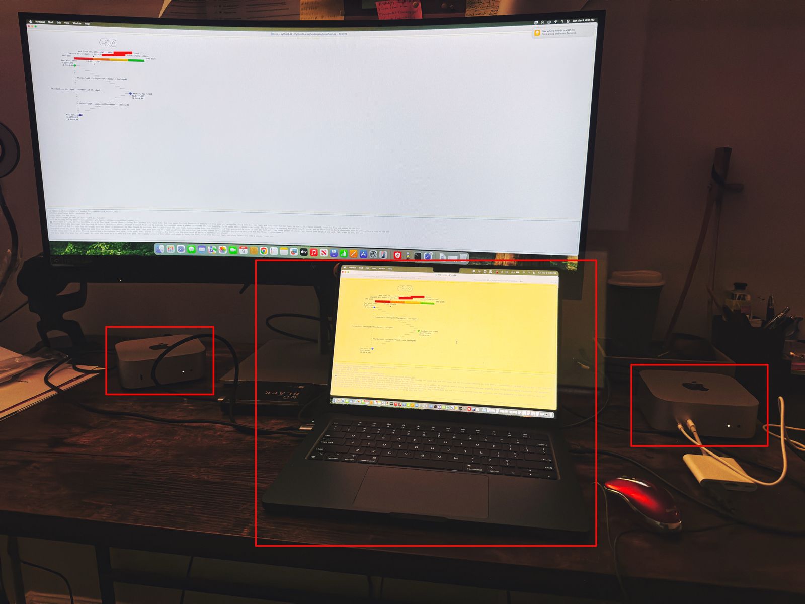
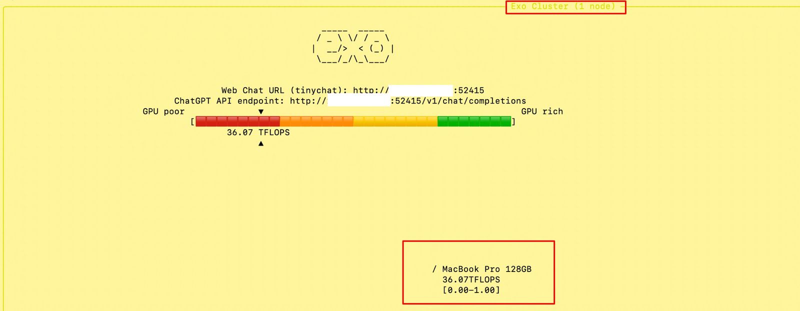
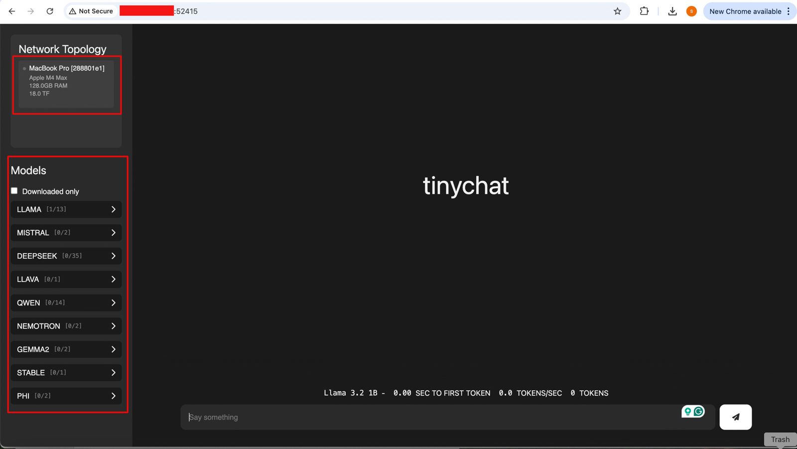


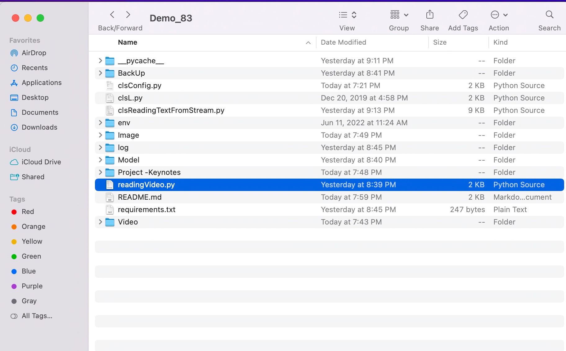

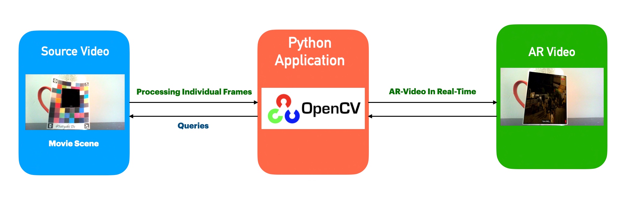


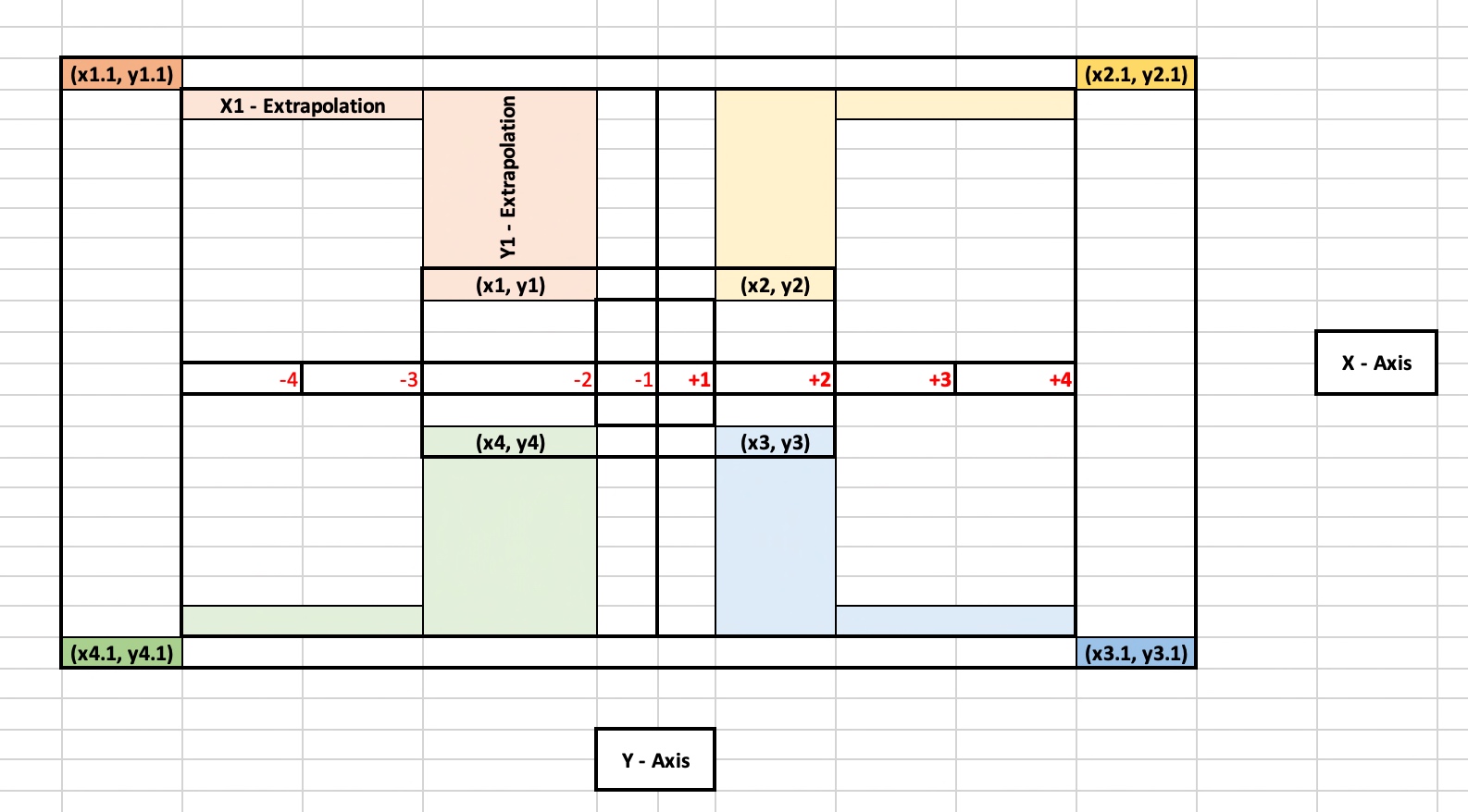


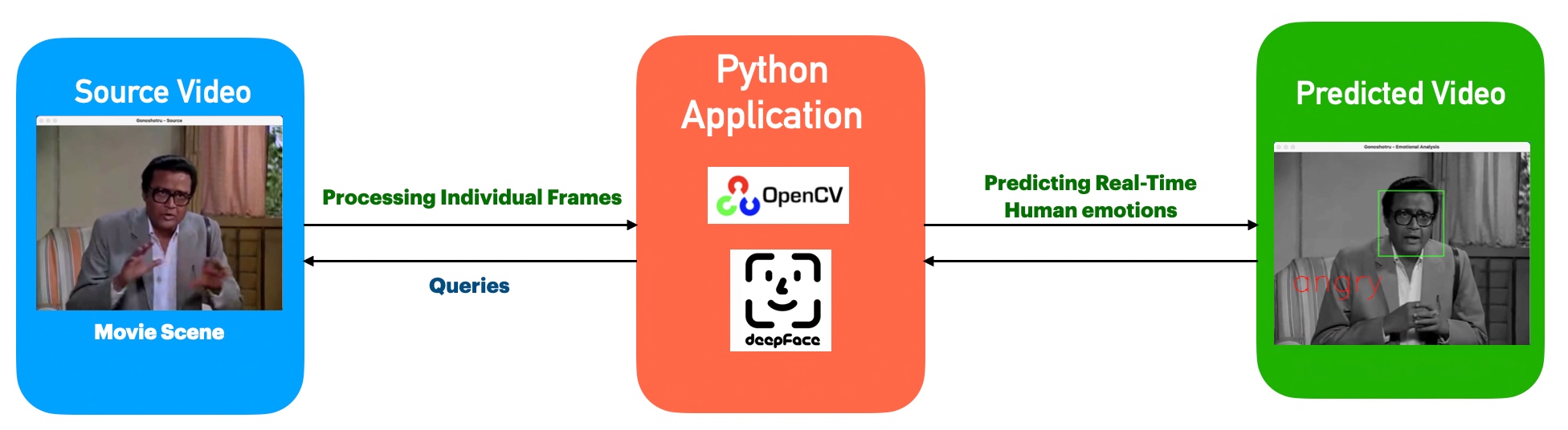

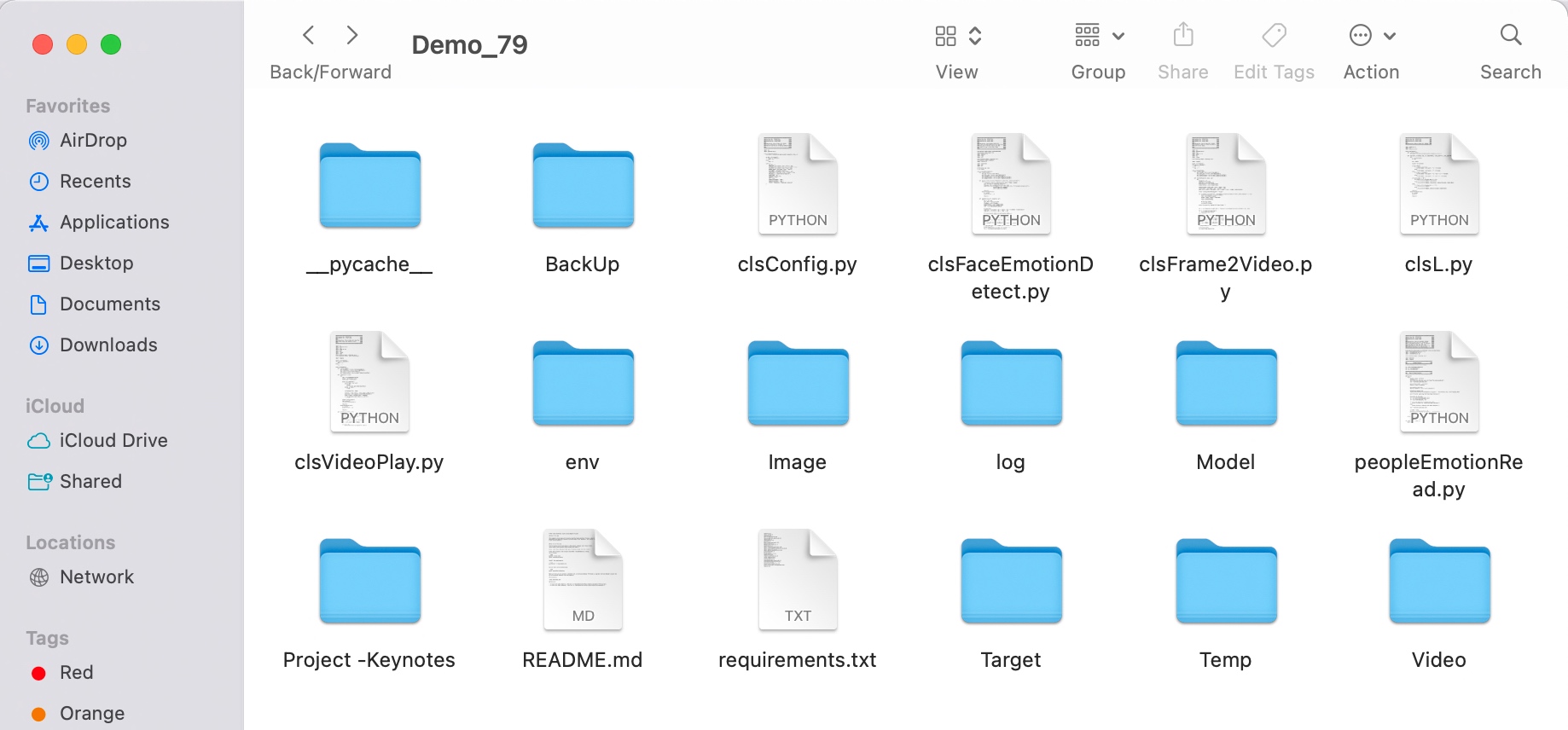


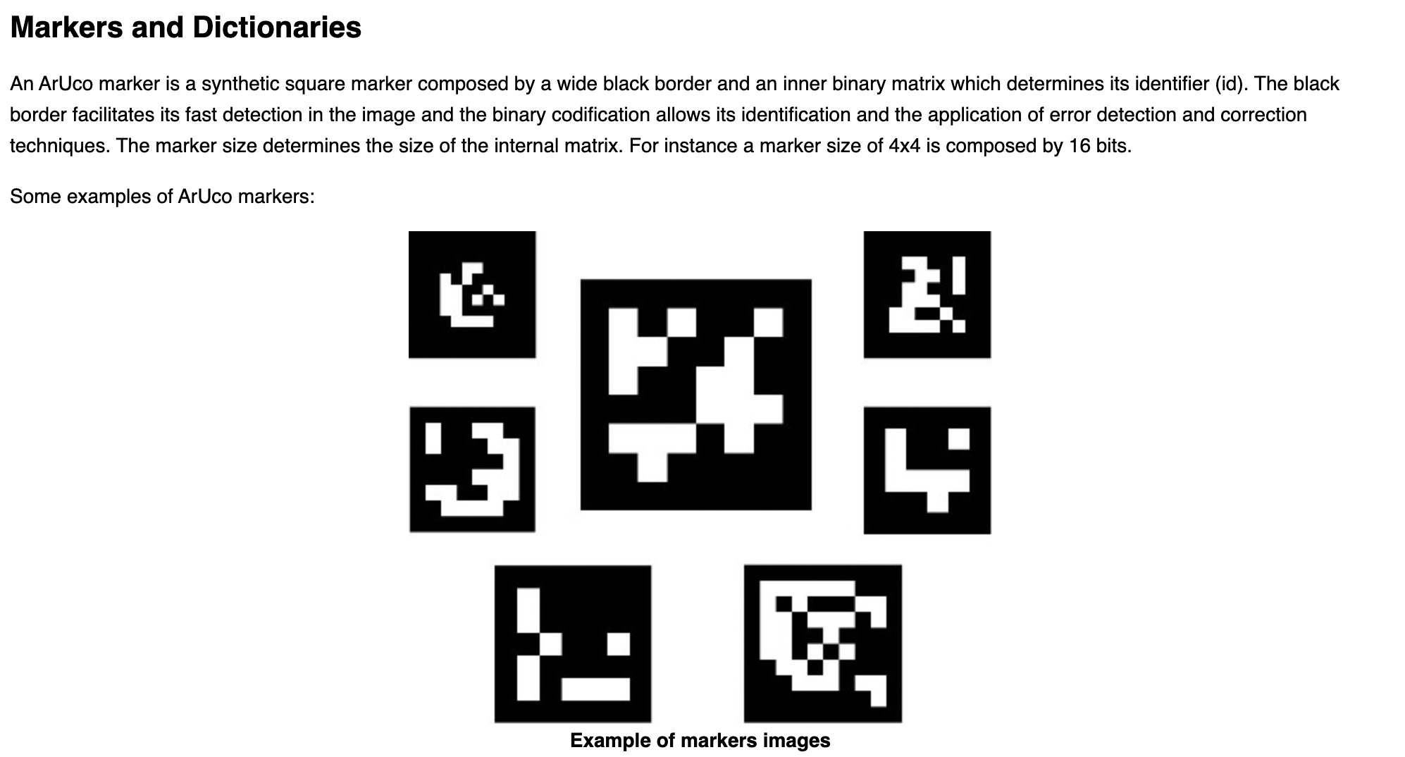


You must be logged in to post a comment.